Updated August 16, 2023
AND Function in Excel (Table of Contents)
Excel AND Function
The AND function is a logical function used when we need to verify two or more values or fields at the same time. AND Function returns the FALSE if any of the used logical values is FALSE. If the answer returned is TRUE, it indicates that all the logic used in the AND function is correct. Also, the AND function works best when combined with other conditional functions, such as If and CountIf.
It is the most commonly used logical function alone or in combination with other operators like:
- “IF”
- “OR”
- “NOT”
- < (less than)
- > (greater than)
- = (equal to)
- <= (less than or equal to)
- >= (greater than or equal to)
- <> (not equal to)
It is most commonly used in conditional formatting.
The AND function in Excel tests multiple conditions; up to 255 logical conditions can be used simultaneously (Note: In Excel 2003 version, the function can only handle up to 30 arguments). AND function can operate on text, numbers, or cell references. AND function needs at least two arguments to return a value. A comma separates arguments; In the end, it provides either a ‘true’ or ‘false’ output based on the arguments inside the AND function.
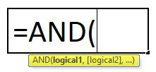
AND Formula in Excel:
Below is the AND Formula in Excel.
logical1: logical value to evaluate, it’s a first condition to evaluate
logical2: logical value to evaluate, it’s a second condition to evaluate
How to Use the AND Function in Excel?
This AND function in Excel is very simple and easy to use. Let us now see how to use AND function in Excel with the help of some examples.
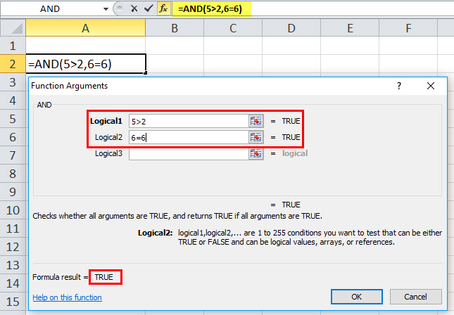
Example #1
If we enter =AND (5>2, 6=6) in an Excel cell, the answer or formula result would be TRUE. It’s true because 5 is greater than 2 and 6 does equal 6.
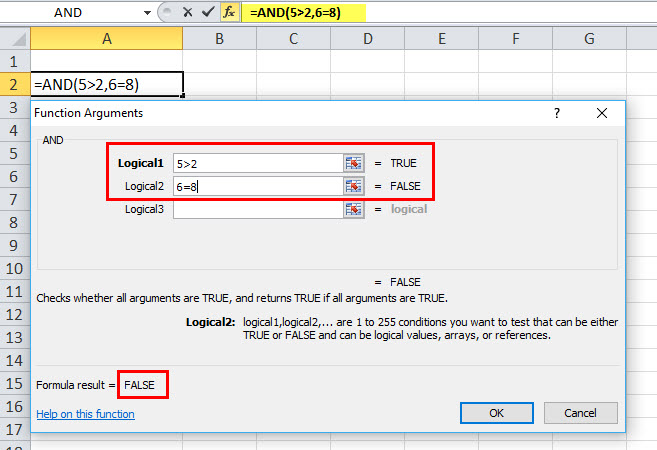
Example #2
If we enter =AND (5>2, 6=8) in an Excel cell, the answer or formula result would be FALSE. It’s false because 5 is greater than 2, but 6 is not greater than 8
NOTE:
- In the AND function formula, each term inside the parentheses is separated by a comma like other functions in Excel.
- If an array or reference argument contains text or empty cells, those values will be ignored.
- Suppose the specified range includes no logical values AND returns the #VALUE! error value.
Example #3
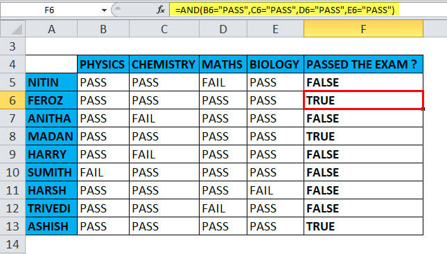
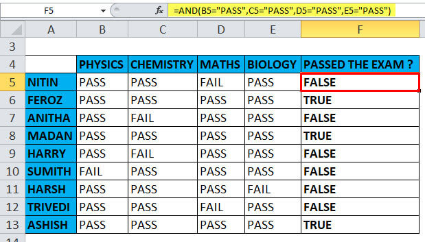
In this example, if a student passes all the subjects, then he has passed the exam
=AND (B6=”PASS”, C6=”PASS”, D6=”PASS”, E6=”PASS”)
The text strings stored in columns B, C, D & E must be “PASS”. Each term inside the parentheses needs to be separated by a comma like other functions in Excel; here, it returns the value TRUE if all of the arguments evaluate TRUE. i.e., if students have passed all the subjects, it returns the value TRUE,
otherwise, even if the students have failed in any of the one subjects, it returns the value FALSE
Example #4
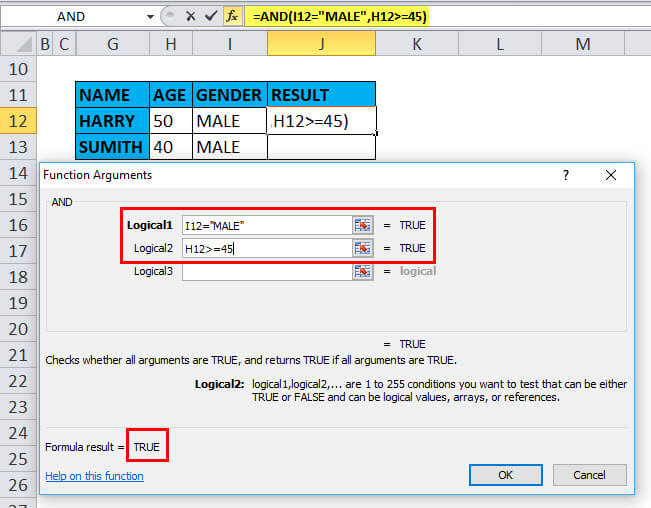
Using other operators (> (greater than) = (equal to) along with AND Function
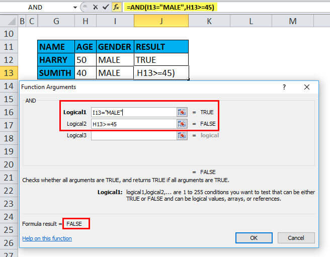
AND function returns TRUE if the first logical condition, Gender parameter I12 = MALE, and the second logical condition, age parameter should be equal to or more than 45 years, i.e., H12>=45. else it returns FALSE. Herewith reference to HARRY, it returns the value TRUE,
In the case of other candidates, SUMITH returns the value FALSE.
Example #5
Using AND with the “IF” Function with other operators
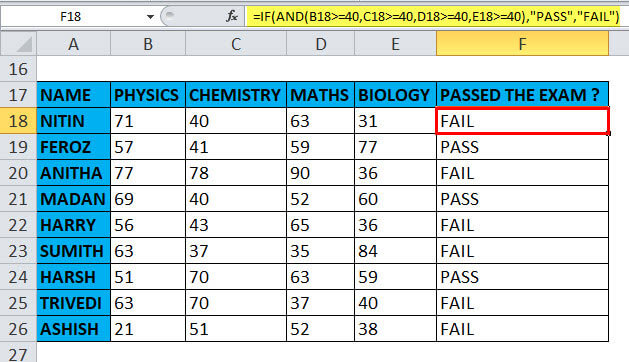
Suppose you have a table with the various subject scores; you need to find out the exam results and whether they have passed the exam.
The first score, stored in column B with the first subject, must be equal to or greater than 40. The second score, listed in column C with the second subject, must be similar to or greater than 40. Similarly, the third & fourth scores, with the third & fourth subjects stored in columns D & E, must be equal to or greater than 40. For a student to pass the exam, all four conditions must be met.
The easiest way to make a proper IF/AND formula is to initially write down the condition first and later add it to the logical test argument of your IF function:
Condition: AND(B18>=40, C18>=40, D18>=40, E18>=40)
IF/AND formula: =IF( AND(B18>=40, C18>=40, D18>=40, E18>=40), “PASS”, “FAIL”)
Example #6
Using AND function with “OR” FUNCTION
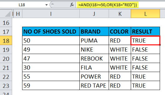
Using IF and AND together is quite simple; in the below-mentioned example, irrespective of brand, in the table array, we need to find out the sales of red color shoes which are more than 50 numbers by using AND with the “OR” function.
The first column contains the number of shoes sold; the second column contains the brand of shoes, and the third column contains the color of the shoes; here, the condition is data in the I column should be equal to, or more than 50 & simultaneously, the color of the shoes should be red.
When both conditions are met, the function returns the value “TRUE”; otherwise “FALSE.”
Recommended Articles
This is a guide to AND Function in Excel. Here we discuss the AND Formula in Excel and how to use AND in Excel as practical examples and downloadable Excel templates. You can also go through our other suggested articles –
