Updated July 5, 2023
TRIM in Excel
The trim in Excel removes the extra spaces from the start and end of the cell value. This is useful when we have the same values in a column, but some cells contain extra spaces. By this Trim function, we can remove the extra spaces from any cell, irrespective of the number of spaces in that selected cell.
TRIM Formula in Excel
Below is the TRIM Formula in Excel:

Trim function arguments
There is only one argument in the Trim function, which is below mention.
=Text(Cell Value / Text)
Shortcut of using the formula
Click on the cell where you want to result in value, then put the formula as below mentioned
= Trim(Cell Value / Text)
Steps for using the Trim function in Excel
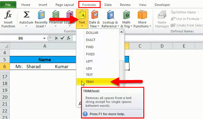
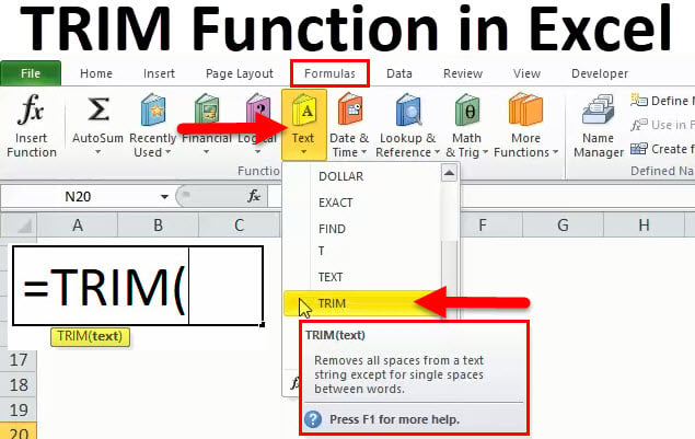
- Click on the formula tab > Text > click on Trim
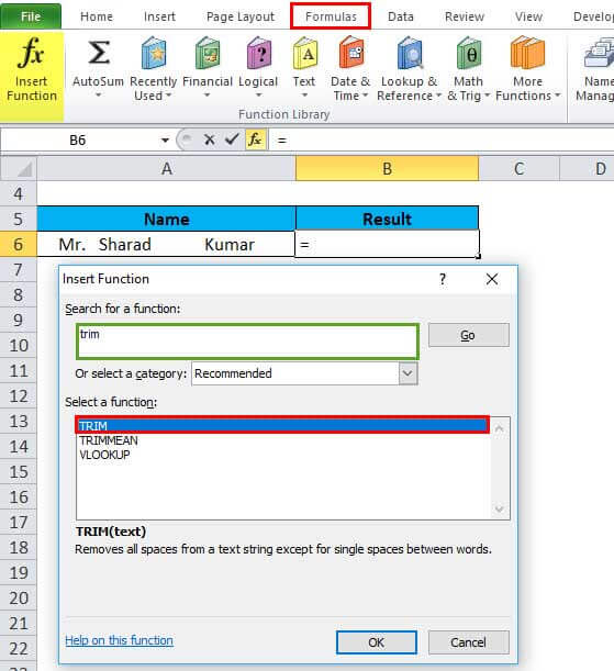
- Also, click on the function icon, then manually write and search the formula.
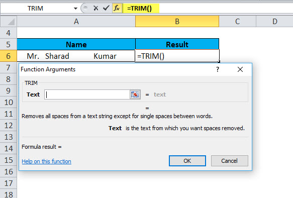
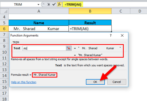
- We get a new function window shown below, mention in the pictures.
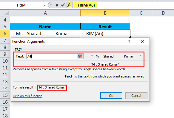
- Then we have to enter the details as shown in the picture.
Put the Cell or text values where you want to remove space from data.
- Then Click On OK.
- The result is:
How to Use the TRIM Function in Excel?
Trim Function in Excel is very simple and easy to use. Let us now see how to use the TRIM function in Excel with the help of some examples.
Example #1
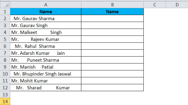
Suppose we have a column of customer names that have some space before and after the text and more than one space between the words. So, how do we remove all extra space in a cell at a time on overall data by copying an Excel TRIM formula across the column and then replacing formulas with their values? Let’s start to write the formula; the detailed steps are mentioned below:
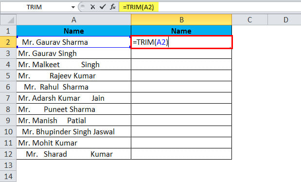
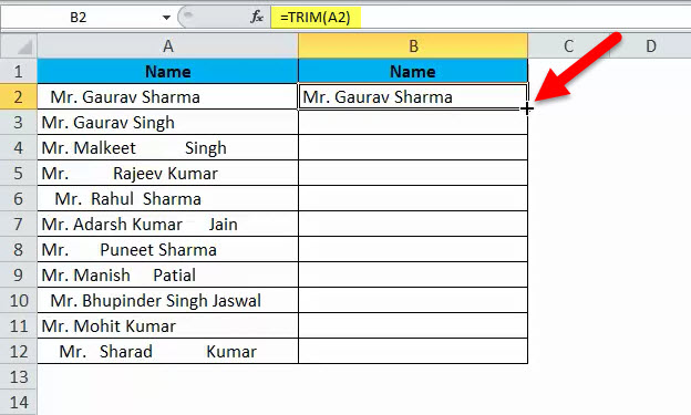
- Write a TRIM formula for the first-row cell, A2, in our example:
=TRIM(A2)
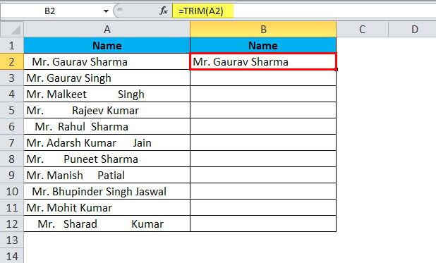
The Result is:
- A position of the cursor to the lower right corner of the formula cell (B2 in this example),
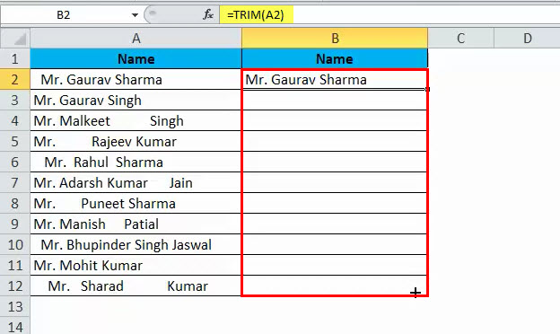
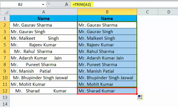
- Select the range (B2:B12) and fill the formula to the last cell with data.
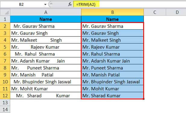
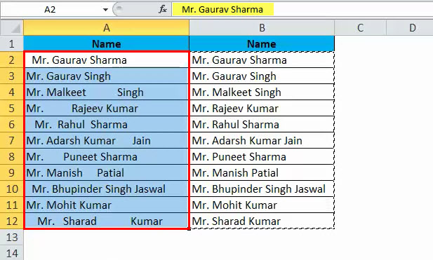
- As a result, you will have 2 columns of original names with spaces and formula-trimmed customers’ names.
Now, replace the values in the original column with the trimmed data value, But be careful. Simply copy and paste the trimmed column data value over the original column; otherwise, destroy your formulas, and we also lose the data. So such a type of this happens. You need to copy only values, not formulas. The steps are below mention.
- Select all cells with Trim formulas (B2:B12 in this example), and copy (CTRL+C) the selected range.
- Select all cells with the original data (A2:A12)
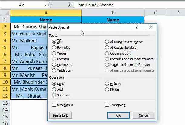
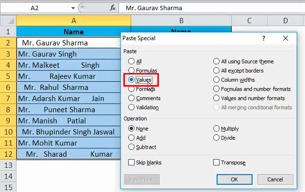
- And Paste the data as value only, not a formula; you can also use a shortcut method for paste special (Ctrl+Alt+V). The dialog box will appear.
- Then again, V is for value.
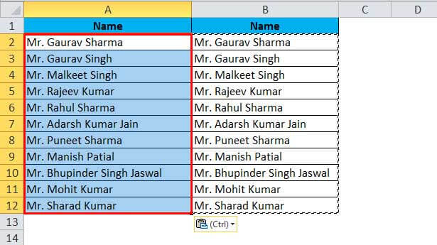
- Press the Enter, and the result will look like
Example #2
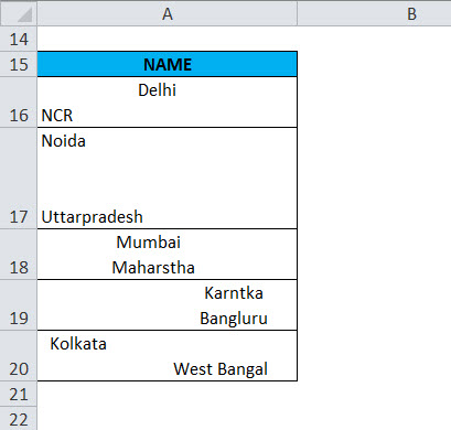
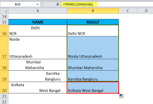
Normally when we fetch data in Excel from another application or any database like SQL Server, Oracle, or HTML, we face such type issue for line breaking with extra space; we can say that double line issue or wrap text issue, and also ever include with a special character which is not removed with only trim. So we can use a trim function with a clean function for such type situations. The example is shown below:
So now we can use a trim function with a clean function.
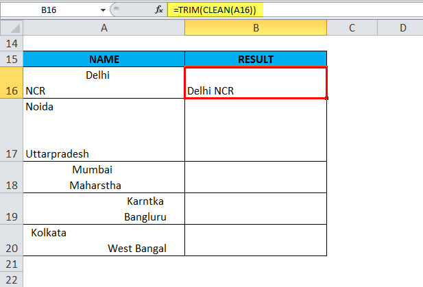
- Write the formula =TRIM(CLEAN(A16))
The result is :
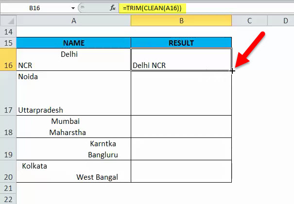
- The cursor is position in the lower right corner of the formula cell (B16 in this example)
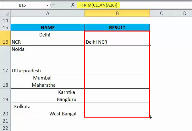
- Select the range and fill down the column with the formula.
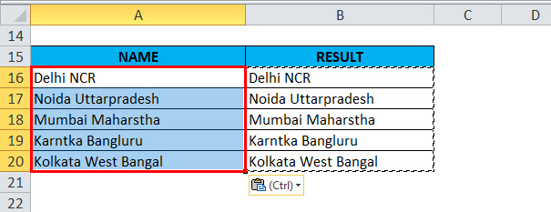
The result is:
- Then you need to copy and paste values only, not formulas like in the first example.
Explanation of the TRIM Function in Excel
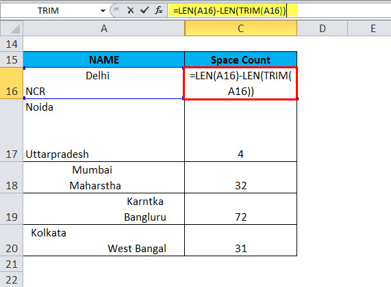
Before removing spaces in data, if we want to know how much extra space or total space is in the Excel sheet, we get the LEN function’s help with a trim function. If you want to get the total number of extra spaces in a cell, then, first of all, we find the total number of text lengths using the Len function, then calculate the string length without extra spaces and subtract the latter from the total length. The formula is as showing below
=LEN(A16)-LEN(TRIM(A16))
The following screenshot shows the above formula in action:
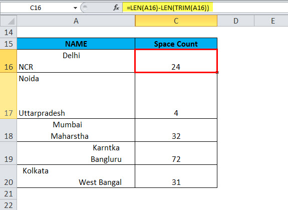
The result is:
Note: This function returns the count of extra spaces in a cell, but this function will not be useful as we want to count with a single space or spaces in the middle of text because trim removed only the unwanted spaces. We can use a substitute formula with the LEN function to get the total number of spaces in a cell.
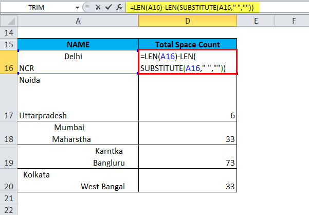
As I remember above, we have used the trim function with a LEN function for extra space count. The same activity we are doing here for total spaces count uses the LEN function with a substitute function. The substitute function replaces old text as a new value; in the example below, we substrates the only text value from the total length count; thus, we found a total no of spaces.
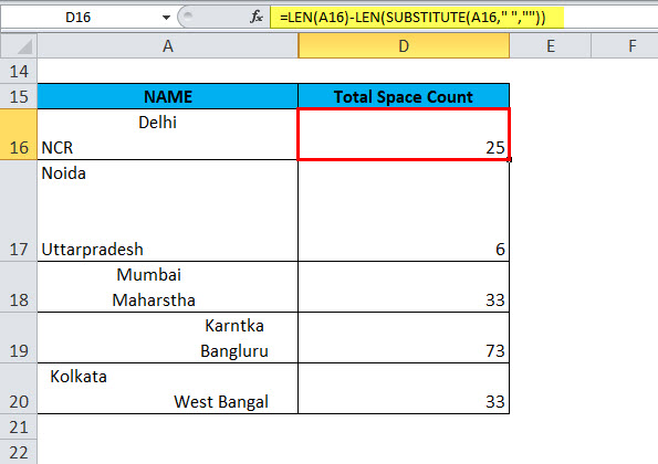
=LEN(A16)-LEN(SUBSTITUTE(A16,” “,””))
The result is:
Things to Remember
- TRIM will remove extra spaces from the text. Thus, it will leave only single spaces between words and no space characters at the start or end of the text.
- The TRIM function was designed to trim the 7-bit ASCII space character (value 32) from the text, so it only removes the ASCII space character (32) from the text.
- The TRIM function will not remove non-breaking space characters commonly used in HTML web pages.
- The Unicode text often contains a non-breaking space character (160) that appears on web pages as an HTML entity. It will not be removed with TRIM.
Recommended Articles
This has been a guide to TRIM in Excel. Here we discuss the TRIM Formula and how to use the TRIM function in Excel, along with practical examples and a downloadable Excel template. You can also go through our other suggested articles –

