TREND in Excel (Table of Contents)
TREND Function in Excel
TREND function is a built-in function in excel which comes under the category of Statistical function to calculate the linear trend line of known y’s and know x’s. TREND function uses the “Least square method to find the line of best fit and to find new y-value for the given x-values. This function is used to predict the future based date where it will be very useful in accounting and financial reporting.
TREND Formula in Excel
The Formula for the TREND Function in Excel is as follows:
TREND Function uses the below arguments as follow:
Known_y’s: The known y’s is a range or array of y values from the line equation.
Known_x’s: The known x’s is a range or array of x values from the line equation. If this x value is null, excel will assume those x_values as 1,2,3..with the same number of values as y values.
New_x ’s: The new_x’s represent the new_x value for which we need to trend to return corresponding values; if the new x argument is null (omitted), it is considered known_x’s value.
Const: The const is a logical value that specifies either “TRUE” or “ FALSE”.
TREND Function:
TREND function is used for multiple values, which are capable of calculating multiple y values and multiple values.
Trend function has four arguments where the first argument is “known y value” and the second argument is “known x value” and the third argument is “ new x values”, and the fourth argument is a constant value which represents “ TRUE” or “FALSE”.
Trend function is an array function that is used to add a trend line to a given chart where we can calculate data and extend the forecast result.
Known_ Y-: This Known y_values is a dependent array or range of data.
Known_ X-: This Known x_values is an independent array or range of data.
New_X-: This new x value is used to return corresponding y values.
Const-: This const is a logical value, i.e. TRUE or FALSE.
Steps of TREND Function in Excel
We can find the TREND Function under Statistical function here; we are going to see step by step procedure on how to use it :
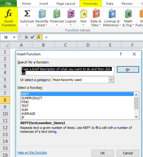
- Choose the insert function, and you will get the below dialogue box, as shown below.
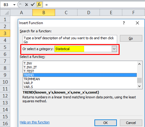
- Select the category statistically; once you choose the category, you will get a list of the function displayed as shown in the below screenshot.
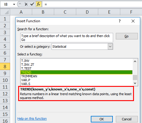
- Select TREND function
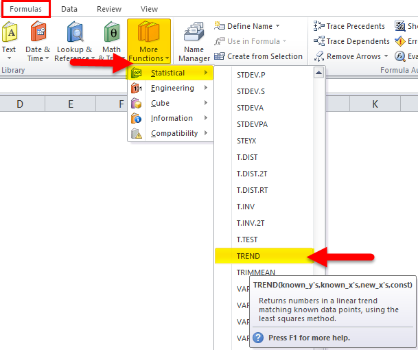
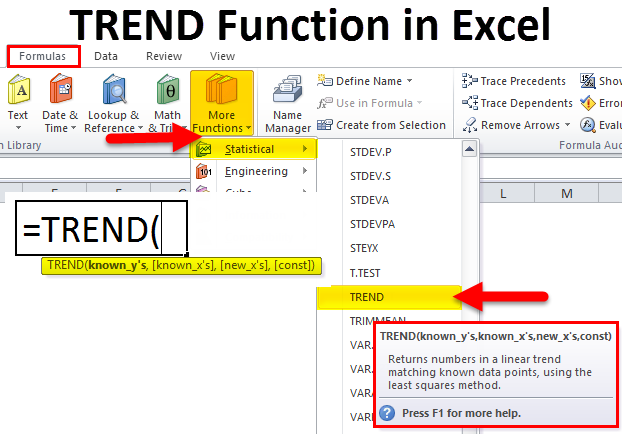
In the advanced version, we will have a shortcut in the formula bar called more function and follow the below procedure.
Go to formulas–>Choose More Function–>Statistical–>TREND
How to use the TREND function in excel?
TREND Function in Excel is very simple and easy to use. Let us understand the working of TREND in Excel by Some Examples.
Example #1
In this example, we have month wise sales data from Jan-18 to Sep-18 where we need to find the next month sales by using the TREND Function in Excel.
Using below TREND Formula.
Here the Trend function with the next month sales has been shown below.
So we have predicted the upcoming sales value for the next three months.
Example #2
Let’s see another example with a graphical chart format using multiple values.
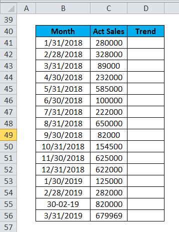
The below example shows months wise sales data where there are ups and downs in sales value; if we produce this format, we cannot view the sales data easily; hence we can show the sales data in using trend function in chart format so that I will be given the appropriate result.
B40 represents Month, C40 represents actual sales, and D40 represents Trend values in the sales data.
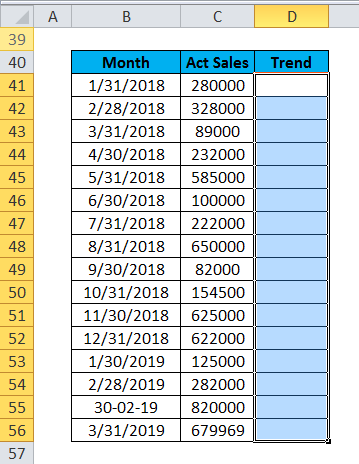
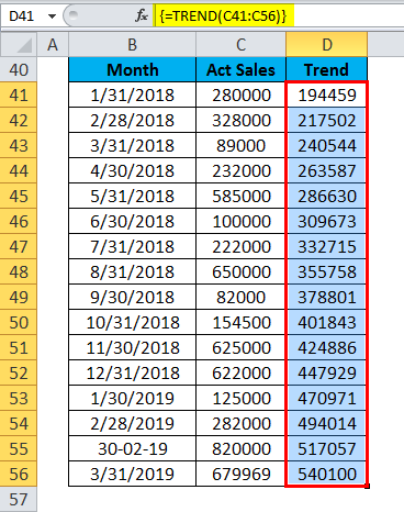
We are going to using the trend function here to get the result, select the column D41 to D56 and use the trend function as per below.
After selection, we use the Trend function by selecting C41: C56 and then we have to use CTRL+SHIFT ENTER to get the entire trend value shown below.
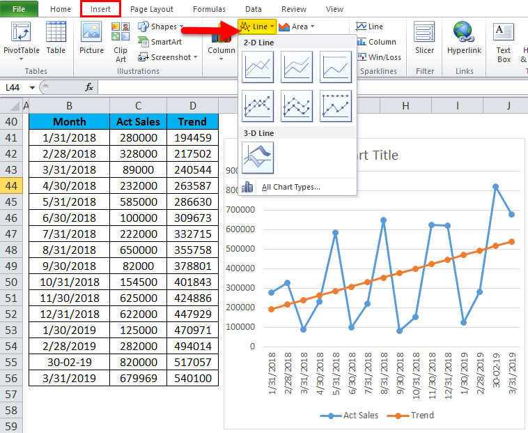
To view in graphical chart format, choose insert and select the line chart format.
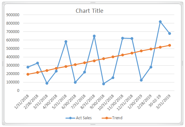
So we get the line chart graph as given below where it shows very clearly sales data month wise.
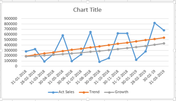
Now, this sales data shows only the trend figure with orange line show linear values, and the graph will be more dynamic if we put the month-wise growth value.
Use the growth function as explained above using CTRL+SHIFT+ENTER; we will get a growth value figure with another line chart which is shown below in grey color.
In sales and financial accounting scenario, these charts are helpful to predict the company production and growth.
Things to Remember About TREND Function in Excel
- Trend Function in Excel helps in determining an array of multiple values.
- In a Business analysis, trend function can be used to analyze revenue, cost, and investment
- FMCG Company can create a trend line of historical sales, and this information can be used to predict the future changes that will be happening in the sales.
- Trend analysis is mainly important in the business, financial, FMCG and other companies to predict future trending sales.
- It is also used in Investment concern to predict the future shares
- In project management, trend analysis is a mathematical technique that uses present data to predict future outcome.
- Trend analysis helps determine that the company is achieving their planned goals, so that management can compare that margin wise sales have reached up or down by performing this trend analysis.
- Used as a real-time and time-based data analysis.
Recommended Articles
This has been a guide to TREND in Excel. Here we discuss the TREND Formula in Excel and how to use TREND Function in Excel along with excel example and downloadable excel templates. You may also look at these useful functions in excel –

