Updated August 16, 2023
Relative Reference in Excel (Table of Contents)
Relative Reference in Excel
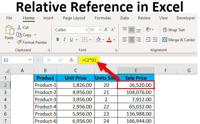
Relative Reference in Excel is like selecting a cell without putting anything in it. By this, the cell value will not be fixed, and whenever we are copying or using that cell, its value will also get changed with the respective Reference of that sheet. For example, the relative Reference of cell A1 will look like “=A1“. This Reference will change when we copy it to other cells or sheets.
What is the Relative Reference in Excel?
Relative references refer to a cell or a range of cells in Excel. Every time a value is entered into a formula, such as SUMIFS, it is possible to input a “cell reference” into Excel as a substitute for a hard-coded number. A cell reference may come in the form B2, where B corresponds to the tcell cell column letter in question and 2 represents the row number. Whenever Excel comes across a cell reference, it visits the particular cell, extracts out its value, and uses that value in whichever formula you’re writing. When this cell reference is duplicated to a different location, the cell’s relative references correspondingly also change automatically.
When we reference cells like this, we can achieve it with any of the two “reference types”: absolute and relative. The demarcation between these two distinct reference types is the inherent behavior of dragging or copying and pasting them into different cells. Relative references can alter themselves and adjust as you copy and paste them; absolute references, contrarily, do not. To successfully achieve results in Excel, it is critical to be able to use relative and absolute references in the right way.
How to Use Relative Reference in Excel?
This Relative Reference is very simple and easy to use. Let us now see how to use Relative Reference in Excel with the help of some examples.
Example #1
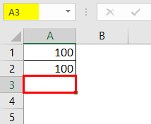
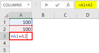
Let us consider a simple example to explain the mechanics of Relative Reference in Excel if we wish to have the sum of two numbers in two different cells – A1 and A2, and have the result in a third cell, A3.
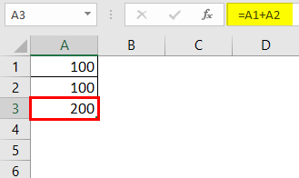
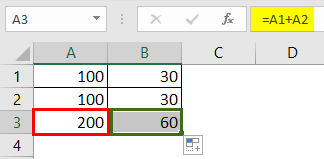
So we apply the formula A1+A2, which would yield the result as 200 in A3.
The result is 200.
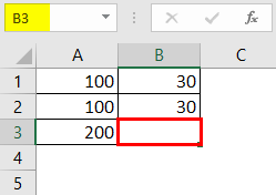
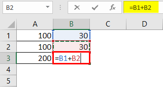
Suppose we have a similar scenario in the next column (“B”). Cell B1 and B2 have two numbers, and we wish to have the sum in B3.
We can achieve this in two different ways:
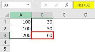
Here we physically write the formula to add the two cells B1 and B2 in B3 to get the result of 30.
The result is 30.
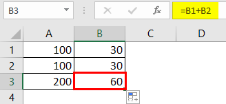
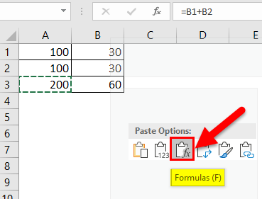
Or we could copy the formula from cell A3 and paste it into cell B3 (it would work if we drag the formula from A3 to B3 also).
So, when we copy the contents of cell A3 and paste them into B3 or drag the contents of cell A3 and paste them into B3, the formula gets copied, not the result. We could achieve the same result by right-clicking on cell A3 and using the Copy option.
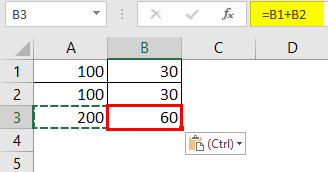
And after that, we move to the next cell, B3, and right-click and select “Formulas (f).”
What this means is that cell A3 = A1+A2. When we copy A3, move one cell to the right, and paste it onto cell B3, the formula automatically adapts and changes to B3 = B1+B2. It applies the summation formula for B1 and B2 cells instead.
Example #2
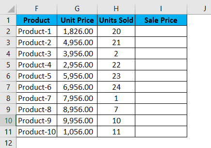
Now, let us look at another practical scenario that would clarify the concept. Let us assume that we have a data co consisting of the unit price of a product and the quantity sold for each. Our objective is to calculate the Sale Price; the following formula can describe price = Unit Price x Units Sold.
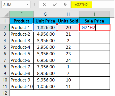
To find the Sale Price, we must multiply the Unit Price with the Units Sold for each product. So, we shall now apply this formula for the first cell in Sale Price, i.e., for Product 1.
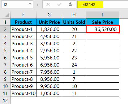
When we apply the formula, we get the following result for Product 1:
It successfully multiplied the Unit Cost by the Units Sold for Product 1, i.e., cell G2 * cell H2, i.e., 1826.00 * 20, which gives us the result 36520.00.
So now we see that we have 9 other products to go. This could go up to hundreds or thousands of rows in real-case scenarios. It becomes difficult to nearly impossible to go about writing the formula for each row simply.
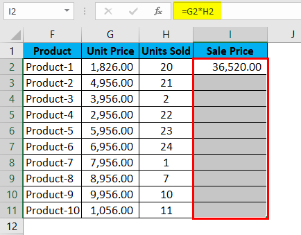
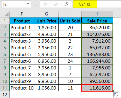
Hence, we will use the Relative Reference feature of Excel and copy the contents of cell I2 and paste in all of the remaining cells in the table for the column Sale Price or simply drag the formula from cell I2 to the rest of the rows in that column and get the results for the whole table in less than 5 seconds.
We can press Ctrl + D or Copy and Paste the cell I2 to all the selected cells.
Things to Remember
- While copying the Excel formulae, relative referencing is generally what is desired. This is the reason why this is the default behavior of Excel. But sometimes, the objective might be to apply absolute Reference rather than relative Reference. Absolute Reference is making a cell reference fixed to an absolute cell address, due to which, when the formula is copied, it remains unaltered.
- Absolutely no dollar signs are required! With Relative referencing, when we copy the formula from one place to another, the formula will adapt accordingly. So, if we type =B1+B2 into cell B3 and then drag or copy-paste the same formula into cell C3, a relative reference automatically adjusts the formula to =C1+C2.
- With Relative referencing, the referred cells automatically adjust themselves in the formula per your movement, either to the right, left, upward, or downwards.
- If we were to give a reference to cell D10 and then shift one cell downwards, it would change to D11; if instead, we shift one cell upwards, it would change to D9. The Reference will change to E10 if we move one cell to the right, and it will automatically change to C10 if we move one cell to the left.
Recommended Articles
This has been a guide to a Relative Reference in Excel. Here we discuss its uses and how to use Relative Reference in Excel with Excel examples and downloadable Excel templates. You may also look at these useful functions in Excel –
