Updated May 10, 2023

Data Filter in Excel
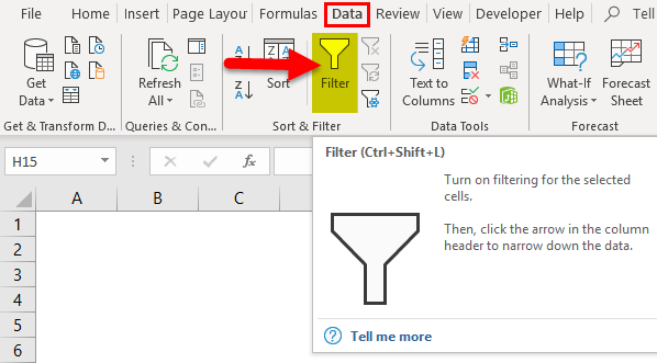
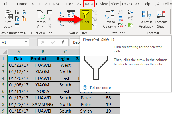
Data Filter in Excel has many purposes apart from filtering the data. Although its main purpose is to filter the data as per the required condition, apart from this, we can sort, arrange the data, and filter the data as per the color of cells or fonts or any condition available in the Text filter in the column where the filter is applied. To apply the filter, first, select the row where we need a filter, then from the Data menu tab, select Filter from the Sort & Filter section. Or else we can apply the filter using the shortcut key ALT + D + F + F simultaneously or Ctrl + Shift + L together.
Uses of Data Filter in Excel
- If the table or range contains many datasets, it isn’t easy to find & extract the precise requested information or data. In this scenario, the Data Filter helps out.
- The data Filter in Excel option helps out in many ways to filter the data based on text, value, numeric, or date value.
- The Data Filter option is very helpful for sorting out data with simple drop-down menus.
- The Data Filter option is significant to temporarily hide a few data sets in a table so that you can focus on the relevant data we need to work on.
- The worksheet applies filters to rows of data.
- Besides multiple filtering options, auto-filter criteria provide the Sort options relevant to a given column.
Definition
Data Filter in Excel: it’s a quick way to display only the relevant or specific information which we need & temporarily hide irrelevant information or data in a table.
To activate the Excel data filter for any data in Excel, select the entire data range or table range and click on the Filter button in the Data tab in the Excel ribbon.
(keyboard shortcut – Control + Shift + L)
Types of Data Filter in Excel
There are three types of data filtering options:
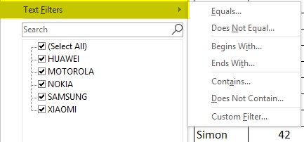
1. Data Filter Based On Text Values – It is used when the cells contain TEXT values; it has below mentioned Filtering Operators (Explained in example 1).
Apart from multiple filtering options in a text value, AutoFilter criteria provide the Sort options also relevant to a given column. i.e. Sort by A to Z, Sort by Z to A, and Sort by Color.
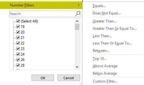
2. Data Filter Based on Numeric Values – It is used when the cells contain numbers or numeric values
It has below mentioned Filtering Operators (Explained in example 2)
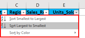
Apart from multiple filtering options in Numeric value, AutoFilter criteria provide the Sort options also relevant to a given column. i.e. Sort by Smallest to Largest, Sort by Largest to Smallest, and Sort by Color.
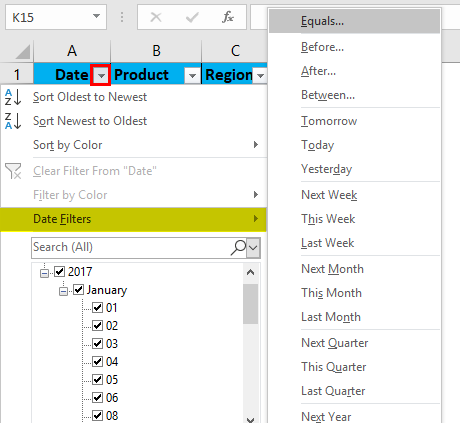
3. Data Filter Based On Date Values – It is used when the cells contain date values (Explained in example 3)
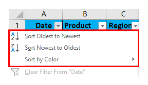
Apart from multiple filtering options in date value, AutoFilter criteria provide the Sort options also relevant to a given column. i.e. Sort by Oldest to Newest, Sort by Newest to Oldest, and Sort by Color.
How to Add Data Filter in Excel?
This Data Filter is very simple easy to use. Let us now see how to Add a Data Filter in Excel with the help of some examples.
Example #1 – Filtering Based on Text Values or Data
In the below-mentioned example, the Mobile sales data table contains a huge list of datasets.
Initially, I must activate the Excel data filter for the Mobile sales data table in Excel, select the entire data range or table range, and click the Filter button in the Data tab in the Excel ribbon.
Or click (keyboard shortcut – Control + Shift + L)
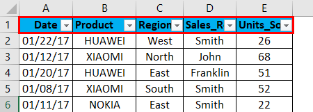
When you click on Filter, each column in the first row will automatically have a small drop-down button or filter icon added at the right corner of the cell i.e.
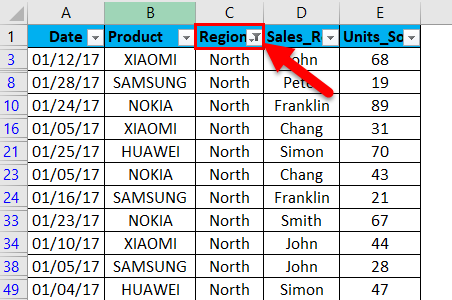
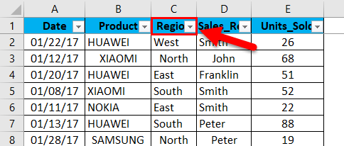
When Excel identifies that the column contains text data, it automatically displays the option of text filters. In the mobile sales data, if I want sales data in the northern region only, irrespective of date, product, sales rep & units sold. I must select the filter icon in the region header; I have to uncheck or deselect all the regions except the north region. It returns mobile sales data in the northern region only.
Once a filter is applied in the region column, Excel pinpoints that the table is filtered on a particular column by adding a funnel icon to the region column’s drop-down list button.
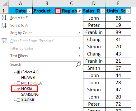
I can further filter based on brand & sales rep data. Now with this data, I further filter in the product region where I want the sales of the Nokia brand in the north region only, irrespective of the sales rep, units sold & date.
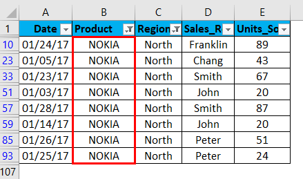
I have to just apply the filter in the product column apart from the region column. I have to uncheck or deselect all the products except the NOKIA brand. It returns Nokia sales data in the north region.
Once the filter is applied in the product column, Excel pinpoints you that table is filtered on a particular column by adding a funnel icon to the product column’s drop-down list button.
Example #2 – Filtering Based on Numeric Values or Data
When excel identifies that the column contains NUMERIC values or data, it automatically displays the option of text filters.
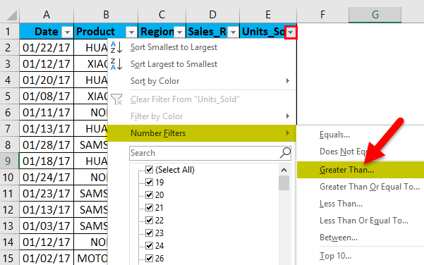
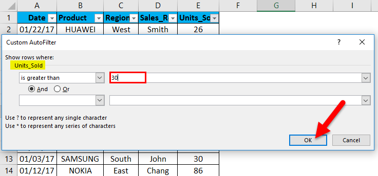
If I want data of units sold in the mobile sales data, which is more than 30 units, irrespective of date, product, sales rep & region. For that, I need to select the filter icon in the units sold header; I have to select the number of filters, and under that greater than an option.
Once greater than option under number filter is selected, pop up appears, i.e. Custom auto filter, in that under the unit sold, we want datasets of more than 30 units sold, so enter 30. Click ok.
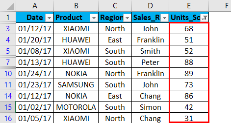
It returns mobile sales data based on the units sold. i.e. more than 30 units only.
Once the filter is applied in the units sold column, Excel pinpoints you that table is filtered on a particular column by adding a funnel icon to the units sold column drop-down list button.
Sales data can be further Sorted by Smallest to Largest or Largest to Smallest in units sold.
Example #3 – Filtering based on Date Value
When Excel identifies that the column contains DATE values or data, it automatically displays the option of DATE filters.
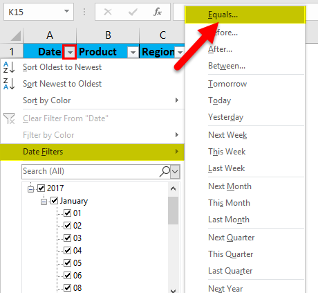
The date filter lets you filter dates based on any date range. For example, you can filter conditions such as dates by day, week, month, year, quarter, or year-to-date.
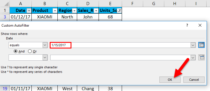
In the mobile sales data, if I want mobile sales data only on or for the date value, i.e., 01/15/17, irrespective of units sold, product, sales rep & region. I need to select the filter icon in the date header; I have to select the date filter, and under that equals to option.
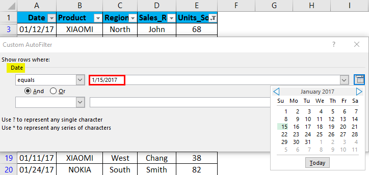
Custom AutoFilter dialog box will appear; enter a date value manually, i.e. 01/15/17
Click ok. It returns mobile sales data only on or for the date value, i.e. 01/15/17
Once a filter is applied in the date column, Excel pinpoints that the table is filtered on a particular column by adding a funnel icon to the date column drop-down list button.
Things to Remember
- Data filter helps specify the required data you want to display. This process is called “Grouping of data,” which helps better analyze your data.
- Excel data can also use to search or filter a data set with a specific word in a text with the help of a custom auto filter on the condition it contains ‘a or any relevant word of your choice.
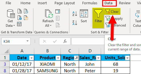
- The data Filter option can remove with the below-mentioned steps:
Go to the Data tab > Sort & Filter group and click Clear.
A Data Filter option is Removed.
- Excel data filter option can filter the records by multiple criteria or conditions, i.e., by filtering multiple column values (more than one column) explained in example 1.
- Excel data filter helps out to sort out blank & non-blank cells in the column.
- data can filter out with the help of wild i.e by changing the question mark. (question mark) & * (asterisk) & ~ (tilde)
Recommended Articles
This has been a guide to a Data Filter in Excel. Here we discuss how to Add a Data Filter in Excel with excel examples and downloadable excel templates. You may also look at these useful functions in Excel –

