Updated August 19, 2023
Highlight Duplicates in Excel
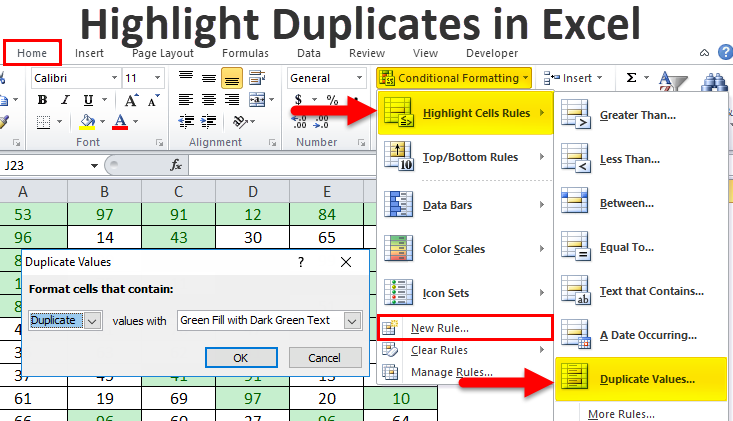
We can highlight the duplicate values in the selected dataset, whether a column or row of a table, from the Highlight Cells Rule, available in Conditional Formatting under the Home menu tab. To highlight the duplicates, select the data from where we need to highlight the duplicates, then select the Duplicate Values option, which is there under Conditional Formatting. From the box of Duplicate Values, choose Duplicate with the type of color formatting we want. Mainly Red text is selected by default to highlight duplicates. In this article, we will learn about Highlight Duplicates in Excel
There are various ways to find duplicate values in Excel. They are:
- Conditional Formatting – Using Duplicate Values Rule
- Conditional Formatting – Using Excel Function or Custom Formula (COUNTIF)
How to Highlight Duplicate Values in Excel?
Highlighting Duplicate Values in Excel is very simple and easy. Let’s understand how to find and highlight duplicate values in Excel using two methods.
Conditional Formatting – Duplicate Values Rule
Here we will find the duplicate values in Excel using the conditional formatting feature and highlight those values. Let’s take an example to understand this process.
Example #1
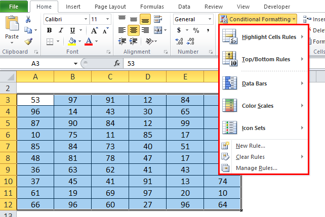
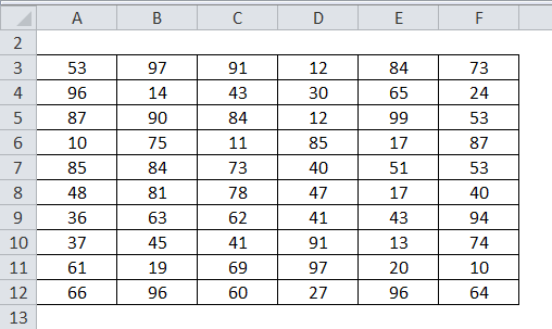
We have given the below dataset.
To highlight the duplicate values in the above dataset, follow the below steps:
- Select the entire dataset.
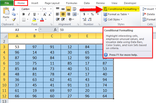
- Go to the HOME tab.
- Click on the Conditional Formatting option under the Styles section, as shown in the below screenshot.
- It will open a drop-down list of formatting options, as shown below.
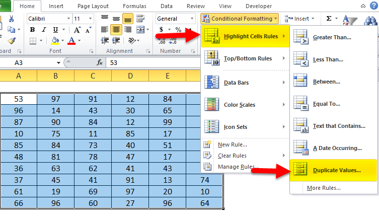
- Click on Highlight Cells Rules here, and it will again display a list of rules here. Choose the Duplicate Values option here.
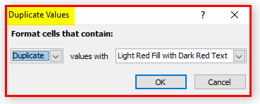
- It will open a dialog box of Duplicate Values, as shown in the below screenshot.
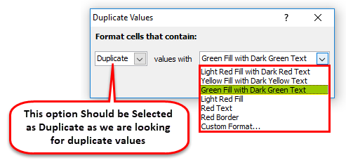
- Select the color from the color palette to highlight the cells.
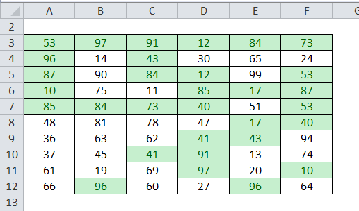
- It will highlight all the duplicate values in the given data set. The result is shown below.
With the highlighted duplicate values, we can take action accordingly.
In the upper section, we highlighted the cells with conditional formatting inbuilt features. We can also do this method by using an Excel function.
Conditional Formatting – Using Excel Function or Custom Formula (COUNTIF)
We will use here COUNTIF function. Let’s take an example to understand this method.
Example #2
Let’s again take the same dataset values to find the duplicate values in Excel.
For highlighting the duplicate values here, we will use the COUNTIF function that returns TRUE if a value appears more than once in the list.
The COUNTIF function we will use like shown below:
=COUNTIF(Cell range, Starting cell address)>1
Follow the below steps to do this.
- Select the whole dataset.
- Go to the HOME tab and click on the Conditional Formatting option.
- It will open a drop-down list of formatting options, as shown below.
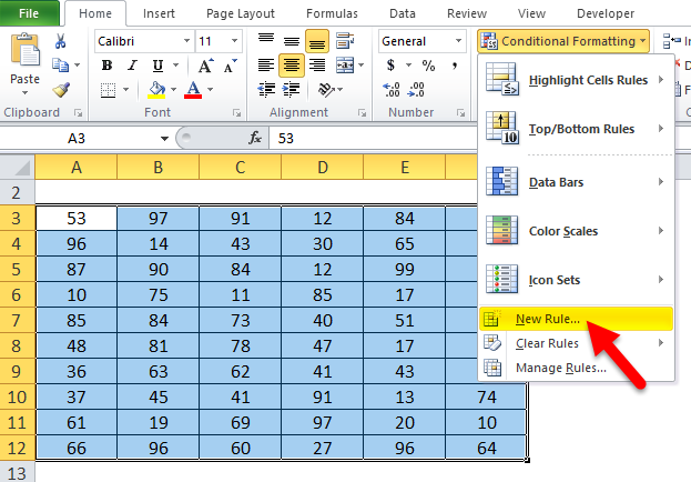
- Click on the New Rule option here. Refer to the below screenshot.
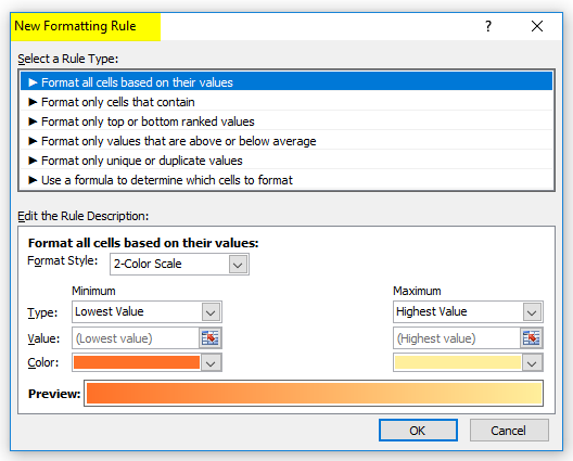
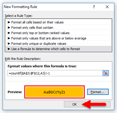
- It will open a dialog box for creating a new custom rule, as shown below.
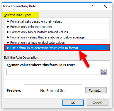
- Select the last option, “Use a formula determining which cells to format,” under the Select a Rule Type section.
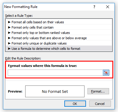
- It will display a formula window, as shown below.
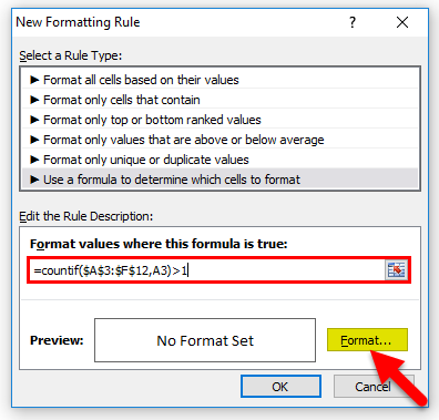
- Enter the formula as =countif($A$3:$F$12,A3)>1, then click on the Format tab.
- Choose the Fill color from the color palette to highlight the cells, then click OK.
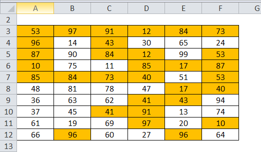
- This will highlight all the cells having duplicate values in the dataset. The result is shown below:
Things to Remember About Excel Highlight Duplicate Values
- Finding and highlighting duplicate values in Excel often comes into use while managing attendance sheets, address directories, or other related documents.
- After highlighting duplicate values, if you delete those records, be extra cautious about impacting your entire dataset.
Recommended Articles
This has been a guide to Highlight Duplicates in Excel. Here we discuss how to highlight duplicate values in Excel using practical examples and a downloadable Excel template. You can also go through our other suggested articles –


