Updated August 16, 2023
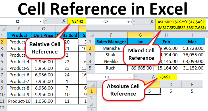
Cell Reference in Excel
Cell Reference in Excel is the way to represent the identity and the location of any cell with the help of combining Column Names and Row Numbers on a worksheet. For example, if we say cell B10, then it expands as Column B and 10th Row. Similarly, we can define or declare cell references to any position in the worksheet. We can also activate R1C1 from Excel Options, another cell reference method, where R1 is Row1 and C1 is Column1.
Types of Cell Reference in Excel
We have three different types of Cell References in Excel –
- Relative Cell Reference in Excel
- Absolute Cell Reference in Excel
- Mixed Cell Reference in Excel
Using the correct type of Cell Reference in a particular scenario will save time and effort and make the work much easier.
#1 – Relative Cell Reference in Excel
Relative cell references in Excel refer to a cell or a range of cells in Excel. Every time you enter a value into a formula, such as SUMIFS, you can input a “cell reference” into Excel as a substitute for a hard-coded number.
. A cell reference may come in B2, where B corresponds to the cell column letter in question and 2 represents the row number. Whenever Excel comes across a cell reference, it visits the particular cell, extracts its value, and uses that value in whichever formula you’re writing. When you duplicate this cell reference in Excel to a different location, the relative cell references automatically change correspondingly.
When we refer to cells like this, we can achieve it with any of the two cell reference types in Excel: absolute and relative. The demarcation between these two distinct reference types is the different inherent behavior when you drag or copy and paste them into different cells. Relative Cell references can alter themselves and adjust as you copy and paste them; absolute references do not. Therefore, to successfully achieve results in Excel, it is critical to be able to use relative and absolute cell references in the right way.
How to effectively use Relative cell reference in Excel?
To comprehensively understand the versatility and usability of this amazing feature of Excel, we will need to look at a few practical examples to grasp its true value.
Example #1
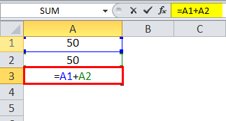
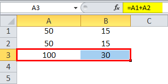
Let us consider a simple example to explain the mechanics of Relative Cell Reference in Excel if we wish to have the sum of two numbers in two different cells – A1 and A2 and have the result in a third cell, A3.
So we apply the formula =A1+A2
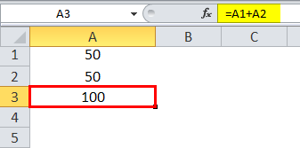
Which would yield the result as 100 in A3.
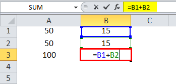
Suppose we have a similar scenario in the next column (B). Cell B1 and B2 have two numbers, and we wish to have the sum in B3.
We can achieve this in two different ways:
Here we physically write the formula to add the two cells B1 and B2 in B3.
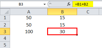
The result is 30.
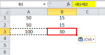
Or we could simply copy the formula from cell A3 and paste it into cell B3 (it would work if we drag the formula from A3 to B3 also).
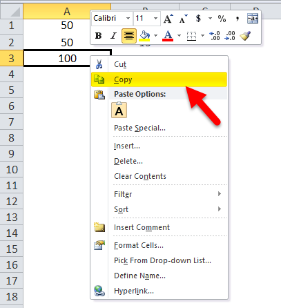
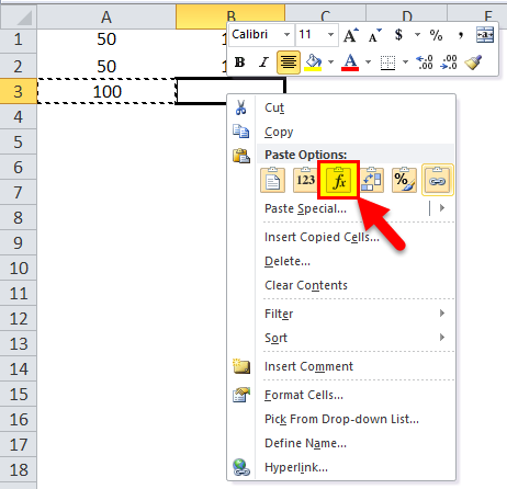
So, when we copy the contents of cell A3 and paste them into B3 or drag the contents of cell A3 and paste them into B3, the formula gets copied, not the result. We could achieve the same result by right-clicking on cell A3 and using the Copy option.
And after that, we move to the next cell, B3, and right-click and select “Formulas (f)”.
What this means is that cell A3=A1+A2. When we copy A3, move one cell to the right, and paste it onto cell B3, the formula automatically adapts and changes to B3=B1+B2. It applies the summation formula for B1 and B2 cells instead.
Example #2
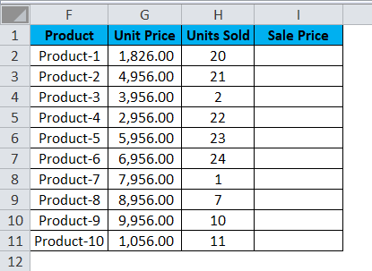
Now, let’s look at another practical scenario that would clarify the concept. Let us assume that we have a data set consisting of the Unit Price of a product and the quantity sold for each of them. Now our objective is to calculate the Sale Price, which the following formula can describe:
Sale Price = Unit Price x Units Sold.
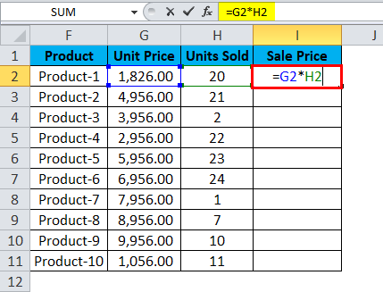
To find the Sale Price, we must multiply the Unit Price by the Units Sold for each product. So, we shall now apply this formula for the first cell in Sale Price, i.e., Product 1.
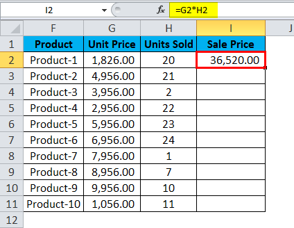
When we apply the formula, we get the following result for Product 1:
It successfully multiplied the Unit Cost by the Units Sold for Product 1, i.e., cell G2 * cell H2, i.e., 1826.00 * 20, which gives us the result 36520.00.
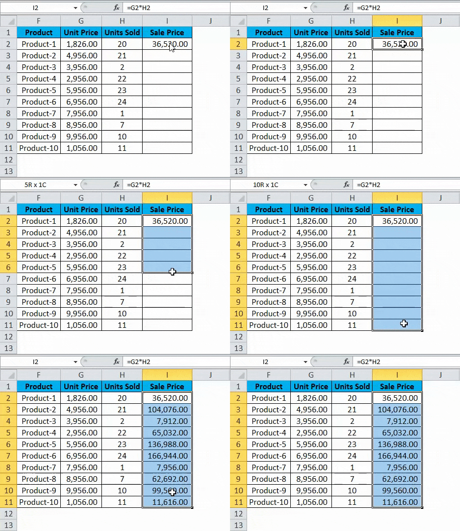
So now we see that we have 9 other products to go. This could go up to hundreds or thousands of rows in real-case scenarios. It becomes difficult and nearly impossible to write the formula for each row simply.
Hence, we will use the Relative Reference feature of Excel and copy the contents of cell I2 and paste in all of the remaining cells in the table for the column Sale Price or simply drag the formula from cell I2 to the rest of the rows in that column and get the results for the whole table in less than 5 seconds.
Here we press Ctrl + D. So the output will look like below
#2 – Absolute Cell Reference in Excel
Most of our daily work in Excel involves handling formulae. Therefore, working with Relative, Absolute, or Mixed cell References in Excel becomes quite important.
Let us see the following:
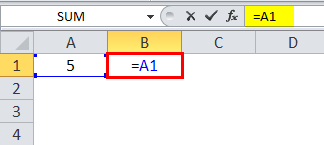
=A1 is a relative reference, where the row and column change when we copy the formula cell.
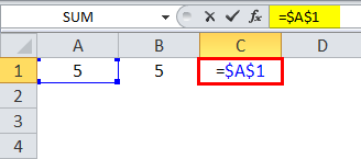
=$A$1 is an absolute cell reference; the column and row are locked and do not change when we copy the formula cell. Thus, the cell value remains constant.
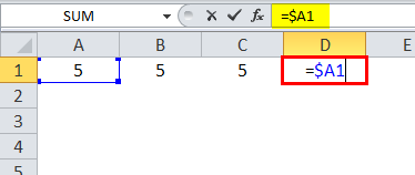
In =$A1, the column is locked, and the row can change for that specific column.
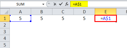
In =A$1, the row is locked, and the column can change for that row.
Unlike Relative Reference, which can change as it moves to different cells, absolute reference doesn’t change. The only thing required here is to lock the specific cell completely.
Using a dollar sign in the formula, w.r.t. a cell reference makes it an absolute cell reference as the dollar sign locks the cell. If the “$” is before an alphabet, it locks a column; if the “$” is before a number, then a row is locked. We can lock either the row or the column using the dollar sign.
#3- Mixed Cell Reference in Excel
How to effectively use Absolute cell reference in Excel and Mixed cell Reference in Excel?
To comprehensively understand Absolute and Mixed cell Reference in Excel, look at the following example.
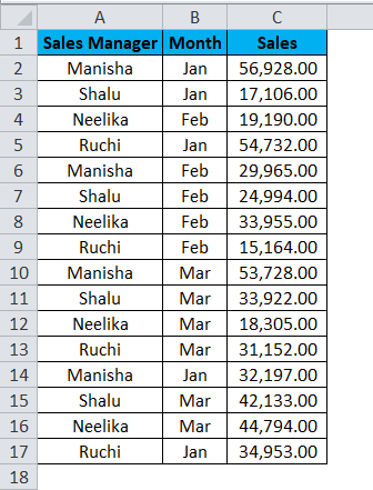
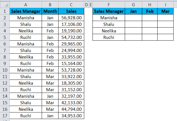
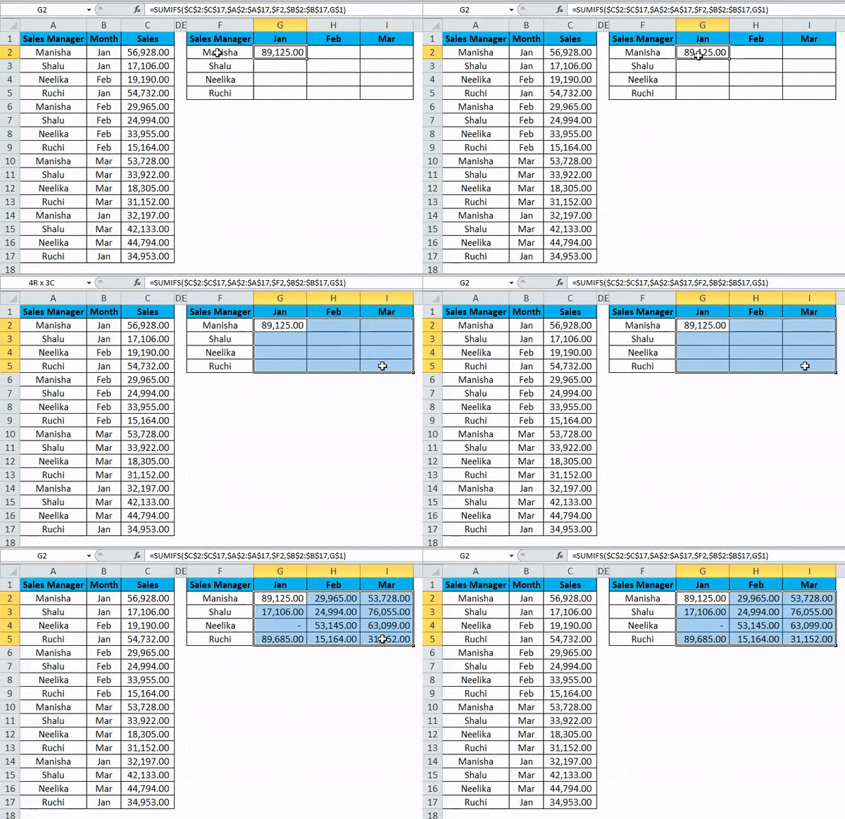
We have the sales data for 4 sales managers across different months, where sales have occurred multiple times a month.
We aim to calculate the consolidated sales summary of all 4 sales managers. We shall apply the SUMIFS formula to get the desired result.
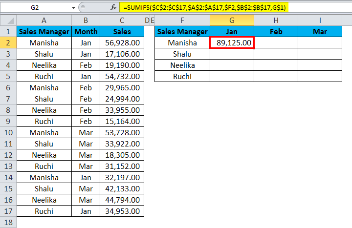
The result will be as follows:
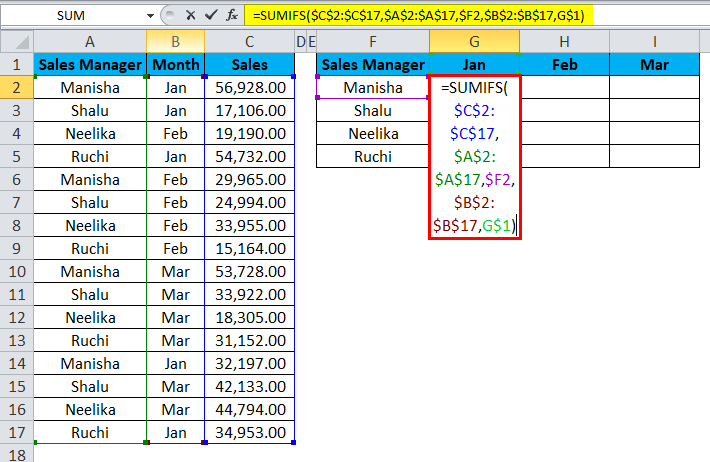
Let us observe the formula to see what happened.
- In the “sum_range”, we have $C$2:$C$17. There is a dollar sign in front of both the alphabet and the numbers. Thus, both the rows and columns for the cell range are locked. This is an absolute cell reference.
- Next, we have “criteria_range1”. Here too, we have absolute cell reference.
- After this, we have “criteria1” – $F2. Here we see that only the column will be locked while copying the formula cell, meaning only the row will change when we copy the formula to a different cell (moving down). This is a mixed cell reference.
- Next, we have “criteria_range2”, also an absolute cell reference.
- The final segment of the formula is “criteria2” – G$1. Here we observe that the dollar sign is in front of the number, not the alphabet. Thus, only the row is locked when we copy the formula cell. The column can change when we copy the formula cell to a different cell (moving right). This is a mixed cell reference.
Dragging the formula across the summary table by pressing the Ctrl+D key first and later Ctrl+R. We get the following result:
Mixed cell reference refers to a row or column, such as =$A2 or =A$2. If we want to create a mixed cell reference, we can press the F4 key on the formula twice to three times per your requirement, i.e., refer to a row or a column. Pressing F4 again will cause the cell reference to change to a relative reference.
Things to Remember
- While copying the Excel formula, you generally desire relative referencing. This is the reason why this is the default behavior of Excel. But sometimes, the objective might be to apply absolute reference rather than relative Cell reference in Excel. Absolute Reference is making a cell reference fixed to an absolute cell address, due to which, when the formula is copied, it remains unaltered.
- Absolutely no dollar signs are required with Relative referencing. When we copy the formula from one place to another, the formula will adapt accordingly. So, if we type =B1+B2 into cell B3 and then drag or copy-paste the same formula into cell C3, the Relative Cell reference would automatically adjust the formula to =C1+C2.
- With Relative referencing, the referred cells automatically adjust themselves in the formula per your movement, either to the right, left, upward, or downwards.
- With Relative referencing, if we were to give a reference to cell D10 and then shift one cell downwards, it would change to D11; if instead, we shift one cell upwards, it would change to D9. If we shift one cell to the right, the reference will change to E10, and instead, if we shift one cell to the left, the reference will automatically adjust itself to C10.
- Pressing F4 once will change the relative Cell reference to the absolute Cell reference in Excel.
- Pressing F4 twice will change the cell reference to a mixed reference where the row is locked.
- Pressing F4 thrice will change the cell reference to a mixed reference where the column is locked.
- Pressing F4 for the fourth time will change the cell reference to the relative reference in Excel.
Recommended Articles
This has been a guide to Cell Reference in Excel. Here we discuss three cell reference types in Excel, i.e., absolute, relative, and mixed cell reference, and how to use each, along with practical examples and a downloadable Excel template. You can also go through our other suggested articles –
