Excel Vlookup from Another Sheet (Table of Contents)
Vlookup from Another Sheet in Excel
VLOOKUP is an Excel function used by Excel users who usually need to work with multiple worksheets. It can extract your data from another worksheet flexibly and organized way. This function takes the user’s input, searches for it in the Excel worksheet, and returns a matching value related to the same information. Speaking technically, the generic definition of the VLOOKUP function is that it looks up a value in the first column of the specified range and returns a similar value in the same row from another column. The VLOOKUP function is available in all versions of Excel, right from Excel 2007 to Excel 2016.
The VLOOKUP function consists of 4 parameters- lookup_value, table_array, col_index_num, and range_lookup. Let us see in detail what these 4 parameters define in the above syntax.
- Lookup_value – Here, the user must define the value that must be searched. It can be either a value that consists of a number, date, or text, or else it can be a cell reference.
- Table_array – Here, the user will define the range of cells they need to search the data. Also, values searched are case sensitive, i.e., it can search for values in the form of text that can be in upper or lower case and find them out.
- Col_index – Here, the value entered refers to the column within the table array where users must find the value.
- Range_lookup – This parameter is optional but is an important parameter to consider. It returns an approximate match if the range lookup value is TRUE and returns exact matches if the range lookup is FALSE.
Example of Vlookup from Another Sheet in Excel
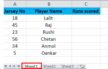
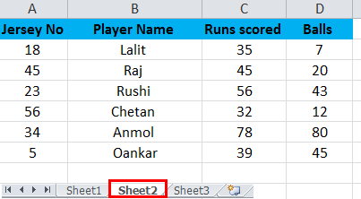
Let us consider an example as shown in the below examples, where we have taken 2 worksheets wherein sheet 1 has players’ names with their jersey numbers but missing runs scored columns. This column needs to be extracted in sheet 1 from sheet 2.
Vlookup from Another Sheet – Example # 1
Vlookup from Another Sheet – Example # 2
As shown in example 2 above, additional columns, such as Columns C and D, are there when compared with sheet 2. We must retrieve data from Column C from sheet 2 to sheet 1. The steps to perform the VLOOKUP function are as follows.
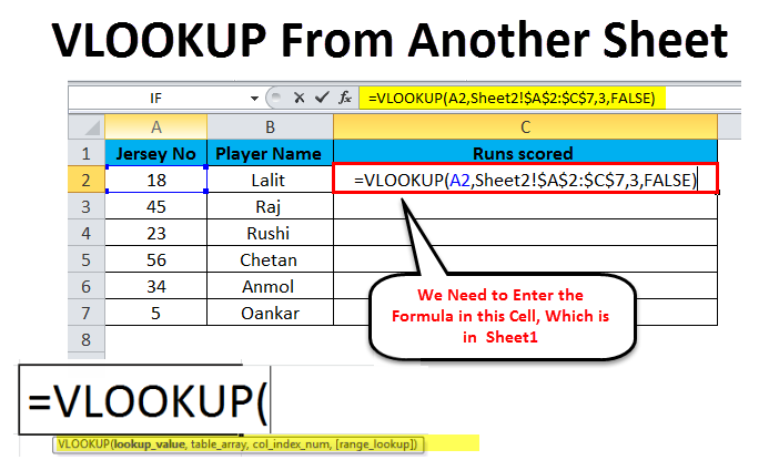
- First, enter the formula =VLOOKUP (A2, Sheet2!$A$2:$D$7,3, FALSE) in cell C2, and press enter.
- We can type the formula in every cell, but copy-pasting will be easier and more efficient.
Let us see the steps below, which will explain the above steps and formula in detail.
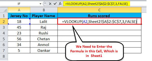
Step – 1
As we can see in above Step1, the formula entered in sheet1 in cell C2 is =VLOOKUP (A2, Sheet2!$A$2:$C$7,3, FALSE) where,
- A2 represents the lookup value of the jersey number, which is the same value in both sheets.
- Sheet 2! is the name of the sheet.
- $A$2:$C$7 is the range of data in sheet2 where we are searching data for the jersey number to fetch the data for runs scored in sheet2. To fix the data range and make it easier to copy and paste in other cells, use the ‘$’ sign.
- 3 is the column index number which contains data in the 3rd column in sheet2 and will retrieve data from the range A2: C7.
- FALSE will return the exact match if the lookup is in range.
Step – 2
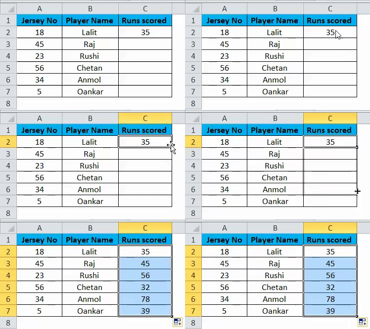
Click on cell C2 and drag down the cell from the corner to apply the formula in all the below cells, as shown in the below image.
The above image is a snapshot of sheet 1, where column C ‘Runs Scored,’ is filled using the VLOOKUP formula.
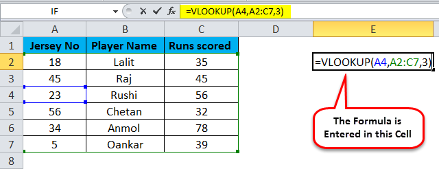
VLOOK function can also be used in the same worksheet, as shown in the below image.
Step – 3
As we can see in Step 3, we have entered the formula in cell E2 to lookup the value for cell C4. A4 is the lookup value; A2: C7 is the search range, i.e., table_array, and 3 is returned matching value from column C. We have not mentioned the sheet’s name in this formula, as we are searching for value in the same sheet.
Step – 4
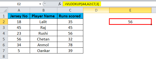
We can see the result returned in the below image.
Advantages of Vlookup from Another Sheet
- This function helps the user search for data in the same sheet or when multiple sheets are in the workbook.
- The VLOOKUP function is much more useful than the MATCH function, as the MATCH function does not return the value of data; it only returns the position of that value.
- VLOOKUP helps the user extract data from one worksheet to another.
- Also, the most important feature offered by the VLOOKUP function is that values can also be looked up from different workbooks.
- It doesn’t matter if you type the text in upper or lower case because the function is not case sensitive. This is a major advantage because it saves time and eliminates the need for the user to worry about the case of the text being searched.
Disadvantages of Vlookup from Another Sheet
- It is tough for a new user to grasp how the formula executes and its parameters.
- If the user performs an approximate match, then the first column of table_array needs to be sorted in ascending order. If not, it will return the correct value. Hence, this function needs to be executed with proper formula knowledge.
Things to Remember
- The VLOOKUP function never searches for the data on the left. It always takes up value for the lookup value in the leftmost top column and starts the search from left to right.
- Always remember when we enter a value less than 1 in the col_index_num parameter, the formula will return an error.
- For an efficient way, use the symbol ‘$’ (absolute cell references) for the table_array parameter so that the user can copy and paste the formula into other cells without any error.
- Also, there is no need to type the entire formula, as when it comes to the part entering the sheet name, you can switch the sheet and select the range using the mouse.
Recommended Articles
This has been a guide to Vlookup from Another Sheet in Excel. The easiest way to adjust a column is to use the Vlookup from Another Sheet in Excel. We discuss using Vlookup from Another Sheet in Excel, practical examples, and a downloadable Excel template. You can also go through our other suggested articles –


