Updated June 9, 2023
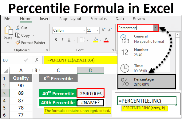
PERCENTILE Formula in Excel
The Percentile is the value for which the percentage of data is forged.
PERCENTILE Formula in Excel calculates the selected array’s specific percentile value. It returns the Kth value. The percentile formula in Excel can be used to find what percentage of values fall under the Kth percentile value.
PERCENTILE function can only be used in Microsoft Excel version 2007 and earlier versions as it is compatible with those versions only. For the latest version or the version which launched later stage of Excel 2007, we can use PERCENTILE.INC or PERCENTILE.EXC gives a more accurate result with the same functional argument compared to Excel’s PERCENTILE formula or function. However, we can use all formats of PERCENTILE in all the latest versions of Excel as well.
How to Use PERCENTILE Formula in Excel?
Using the PERCENTILE Formula in Excel is easy and convenient when calculating n number of percentile for given data. Let’s take some examples to understand the usage of the PERCENTILE Formula in Excel.
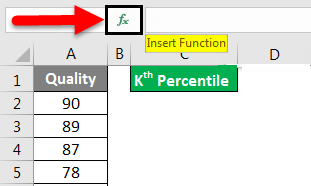
PERCENTILE formula can use from the Insert Function, beside the formula bar, by clicking the Insert Function icon.
Where,
Array = Range of data for which we need to calculate percentile,
k = Percentage value at which we need percentile.
PERCENTILE Formula in Excel -Example #1
We have sample data as shown below, which has a quality percentage of some workers. Where the quality ranges from 1% to nearly 90%, now, with the help of percentile, we will calculate how much percentage of data is marked in which percentile category.
As we can see in the above screenshot, we have a range of qualities for which we need to file the percentile value at any point. Now, go to the cell where we need to see the calculated percentile and select Insert Function near the formula bar, as shown below.
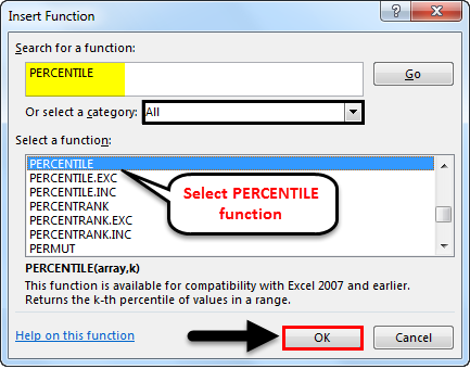
Once we do that, we will get the Insert Function box. Select the PERCENTILE function from All under the Or select a category box or search Statistic. Select the PERCENTILE function from there and click OK, as shown below.
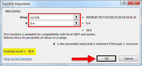
After that, we will get a function argument box of the Percentile function. As we can see, as per syntax here, we must select the Array and the K value. For example, let’s calculate the 40th Percentile. For that, select the array. Here our array range is from cell A2 to A31, and for the K value, enter 0.4 (40% Percentile Criteria). Once we do that, if our defined syntax is correct, we will see the result in the argument box, as shown below. Once done, click on OK to get the result.
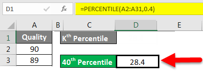
As we can see in the below screenshot, the calculated 40th Percentile is coming as 28.4, which means 28.4% of the selected values are under the 40 Percentile range.
PERCENTILE Formula in Excel -Example #2
There is another method by which we can find the Percentile value at any given percentage range. And in this example, we will see the PERCENTILE.INC function, which Microsoft recommends in place of PERCENTILE with the same syntax but with a more accurate result. For this, we will consider the same data set we saw in Example 1.
Now go to the cell where we need to see the output and type the “=” sign (Equal) to edit that cell’s edit mode. This will enable all the inbuilt functions in Excel. From here, we search for PERCENTILE.INC or PERCENTILE. As we can see in the below screenshot, with the same name Percentile, we got 5 functions. Now select PERCENTILE.INC, which is the substitute for the PERCENTILE function.
Even if we put the cursor on PERCENTILE, INC, it will show us the same significance, reflecting the same for the PERCENTILE function once we select the PERCENTILE.INC, we will see the syntax of it, which is the same as that of the PERCENTILE function, as shown below.
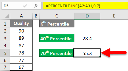
Now for Array, select the complete set of data. Here we are setting the data from cell A2 to A31. And for the K value, let’s consider the 70th percentile; for that, enter 0.7 in a value of K and press enter to see the result.
As we can see in the below screenshot, the calculated 70th Percentile is coming as 55.3, which means 55.3% of the selected values are under the 70 Percentile range.
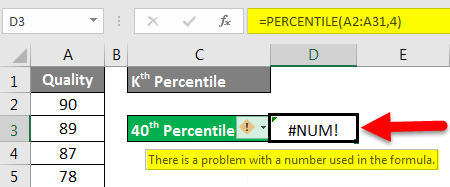
If we enter a whole value in place of a decimal for the K value, we will get an error message, as shown below.
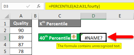
This is the numerical error, which happens when we consider the incorrect numeric reference. And if we enter a text in place of the decimal value, we will get an error message, as shown below.
This alphabetical text error happens when we select an incorrect argument as text. We need to select the percentage in decimal numerical format for the K value, which we have seen in the above examples.
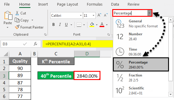
Also, keep the obtained percentile value in its original format. If we change its format into a percentage, it will add an additional 100 digits along with the percentage sign, and the whole purpose of the percentile will be changed, as demonstrated below.
Things to Remember
- If you are using Excel 2013 or higher version, then it is always recommended to use INC in place of PERCENTILE is the advanced and more accurate function with the same syntax to be written.
- K value should always be in decimal so that it will get converted into a percentage in the formula itself.
- The obtained percentile value will already be in Percentage. So it is not recommended to change the value into a percentage. You may add more percentages to the obtained percentile value if you do.
- Percentage and Percentile are both different. Percentile is the value for which the percentage of data is forged, whereas Percentage is completing anything.
Recommended Articles
This has been a guide to PERCENTILE Formula in Excel. Here we discussed How to use PERCENTILE Formula in Excel, practical examples, and a downloadable Excel template. You can also go through our other suggested articles–


