Excel LOOKUP Function (Table of Contents)
Introduction to LOOKUP Function in Excel
The lookup function in excel is used to find the approximate match of any one row or one column as per selection criteria, and it returns the value from the corresponding any one row or one column. This works like Vlookup, but the Lookup function’s major advantage is that it considers both row and column to find the lookup range value.
In simple terms, this function searches the lookup value in a row or a column and gives a matching value in the same location from another cell or column. This is a built-in worksheet function in Excel. So it can be used as a formula in a worksheet. It can be found in Lookup & References under the Formula tab on the ribbon. It is present on all the versions of MS Excel.
Syntax:
The LOOKUP function syntax has two types:
1. Vector
=LOOKUP(lookup-value, lookup-vector, result-vector)
- Lookup Value: It is the value that we want to search in a range or array. It can be a text, number, reference, logical value or a name.
- Lookup Vector: It is a single row or column containing data sorted in ascending order.
Result Vector: It is a single row or column having data and of the same size as the lookup vector.
2. Array
=LOOKUP(lookup_value, array)
- Lookup _value: To search for a value in an array.
- Array: It is the range of cells containing multiple rows and columns where you want to search the lookup value.
The Lookup function searches the lookup value in the Lookup vector and returns the value in the same position from the result vector. The function can return string, numeric, name depending upon the data type.
This function is used for finding prices of products from a data table, transactions from previous months/years, finding marks of students.
How to Use the LOOKUP Function in Excel?
We will now look at how to use the Lookup function with the help of various examples. You will get to know how to write the lookup formula to find the needed values for various criteria.
Example #1
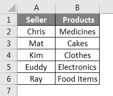
Starting with a basic example using the vector form of the lookup function. We have a sample data table of the seller and their products.
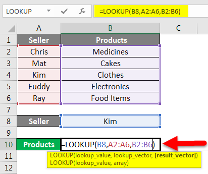
Now, if we want to find out products sold by Kim, we will write the Lookup formula as below:
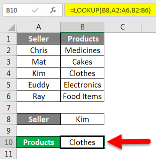
Press Enter to see the result.
We find out that Kim sells clothes.
Explanation of the formula:
=Lookup(B2,A2:A6,B2:B6)
Here B8 (Kim) is the lookup value as we want to know the product sold by her.
A2:A6 is the lookup_vector. We will search for the lookup value in this column.
B2:B6 is the result_vector. It is the column from where the function will return the value.
We wanted to find the product sold by Kim, so first, the function will search Kim in the A2:A6 range and then will return the value in the same position from B2:B6.
Example #2
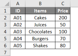
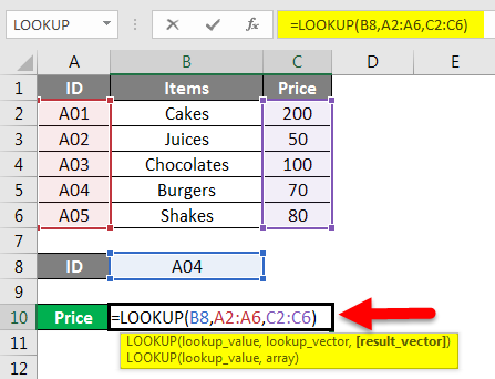
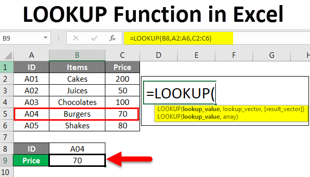
We have s sample data showing ID, Items, and their Price.
Suppose we want to find out the price for ID A04. For this, we will write the formula as below:
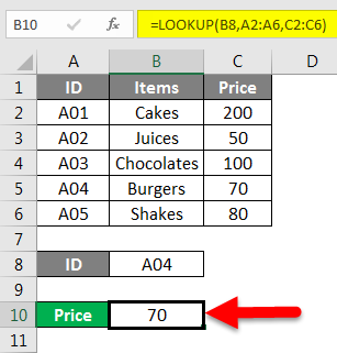
Press Enter to get the result.
The price of ID A04 is 70. Here the lookup value was ID A04; the lookup_vector was A2: A6, and the result_vector was C2: C6. For writing a correct formula, just follow the syntax that is prompted when you start writing the formula.
Example #3
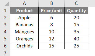
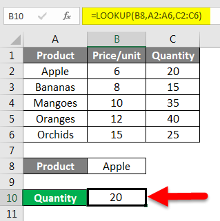
Here we have a data table showing a product, price per unit and quantity.
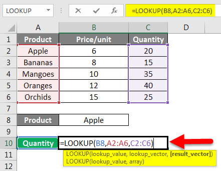
How do we find the number of apples from this table? We can write this formula for this:
Press Enter to see the quantity of apples.
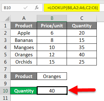
Similarly, we can find out the quantities of other products like Orange.
So with the above examples, you will develop an understanding of the Lookup formula using vector form. Now I will show you a Lookup array example.
Example #4
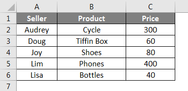
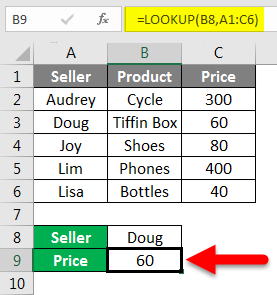
We have this sample data.
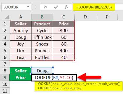
Now, if we want to search the name and pull matching price, how would we do it? Say I want to know the price for the products sold, Doug.
For this, I will write the lookup formula as below:
Press Enter to see the result.
Explanation of the formula:
=LOOKUP(B8, A1:C6)
Here theA10 is the lookup value as we wanted to know the price of the product sold by Doug. The array A1: A6 is the range of cells where we want to search B8. This is how we use the array form of the Lookup function.
Example #5
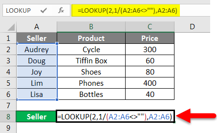
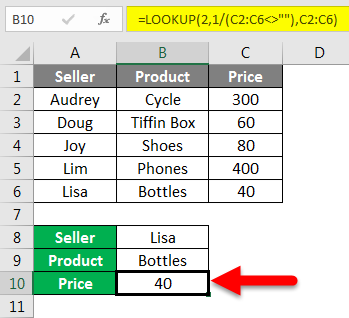
We can also know the last entry for the last entry in a data table’s non-blank column with the Lookup function. Taking the above data table, we can find out how this works.
The syntax is:
=Lookup(2,1/(column<>””), column)
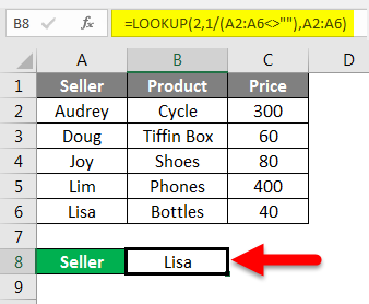
To find the last entry, we will write the formula, as shown below:
Press Enter to see the results.
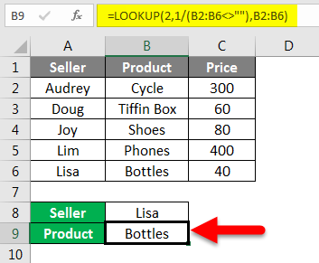
Similarly, we can find the last entries of the Product and Price columns as well.
Now the last entry in the Price column.
Example #6
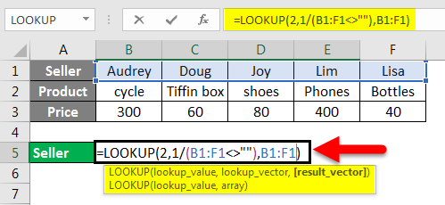
As in our previous example, we found the last entry in a column using the Lookup function. We can also find the last entry in a row. We will write the formula for the same as shown below:
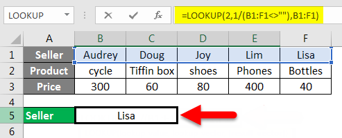
Press Enter.
The syntax is :
= Lookup(2,1/(Row<>””),Row)
Hence the last entry in Seller Row is Lisa. These were some of the most commonly used examples of the Lookup function In Excel.
Things to Remember
- In the Vector form of the Lookup function, the values in Lookup_Vector should be in ascending order. If the values are numeric, they should be sorted from smallest to largest, and if they are in text form, they should be sorted from A to Z.
- The Lookup Function is a case-sensitive function.
- The Lookup_vector and Result_vector should be of the same size.
- In the case of Array Lookup, if the number of columns is more than rows, the lookup function will search the value vertically.
- The Lookup function will give N/A# Error if the lookup_ value is smaller than the smallest value in lookup_vector.
- The same N/A# Error occurs if the lookup_vector is not in ascending order.
- REF# Error occurs when the cell reference does not exist or the cell is deleted after the formula is applied.
Recommended Articles
This is a guide to the LOOKUP Function in Excel. Here we discuss how to use the LOOKUP function for various criteria in Excel along with practical examples and a downloadable excel template. You can also go through our other suggested articles –

