Updated May 9, 2023
Sumif Function Examples (Table of Contents)
Overview of Sumif Function Examples
It adds the values or sum-up cells that meet the given criteria’ expectations.
The Formula for the SUMIF function is:
The SUMIF function syntax or formula has the below-mentioned arguments:
- Range: (Compulsory or required argument) It is the range or array of cells that need to be evaluated by your criteria, e.g., A1:A12
- Criteria: (Compulsory or required argument) It indicates what needs to be added or summed up in a range of cells or which cells to add in a field.
Note:
-
- In the criteria argument, values should always be presented as or enclosed within double quotes.
-
- Because it is case-insensitive, you can present this criteria argument parameter in lower, proper, or upper-case text format.
- sum_range: (Optional parameter or argument) It is an optional array or range of numeric values that must be added.
How to Use SUMIF Function in Excel?
Let’s check out how the SUMIF function works in Excel.
Example#1 – SUMIF Function with Text Criteria
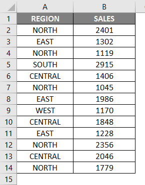
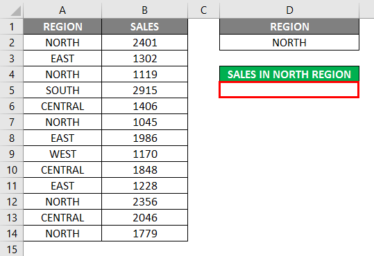
In the below-mentioned example, the table contains a list of regions in column C (C8 to C20) & corresponding sales in that region in column D (D8 to D20). Here I want the sum of sales value in the North region only, i.e., “NORTH” from this sales dataset range (C8 to C20).
Let’s apply the SUMIF function in cell “F11” with an insert function option or type a formula, i.e., =SUMIF automatically the argument which needs to enter appears i.e.
=SUMIF (range, criteria, [sum_range])
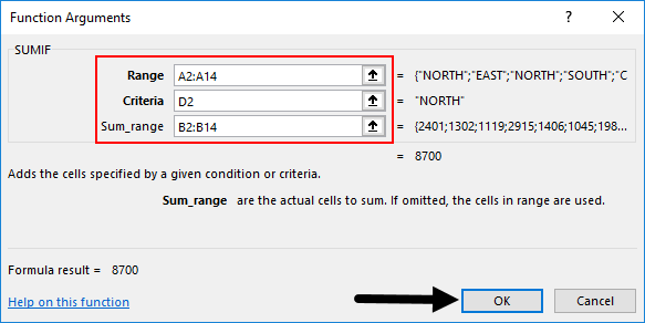
Now the arguments need to be entered i.e.
- Range: Column A is the range or array of cells that need to be evaluated by your criteria, i.e., Here, the range is A2 to A14
- Criteria: It is a parameter or a condition that indicates the SUMIF function in which cells in a range need to be summed or added up; here, I want the sum of sales value for the North region only; hence we need to enter text criteria, i.e., “NORTH.”
- [sum_range]: Column B is an array or range of sales values that must be added. i.e., here, the range is B2 to B14
Click ok after entering all three arguments.
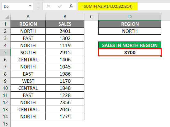
=SUMIF (A2:A14,D2,B2:B14)
i.e., returns the sum of sales value in the north region, i.e., “8700.”
Example #2 – Numeric Values with Arithmetic or Comparison Operators
Various arithmetic operators can be used in the SUMIF function:
> Greater Than
< Less Than
= Equal to
>= Greater than or equal to
<= Less than or equal to
<> Less than or greater than
a. SUMIF Function with Greater Than (>) operator
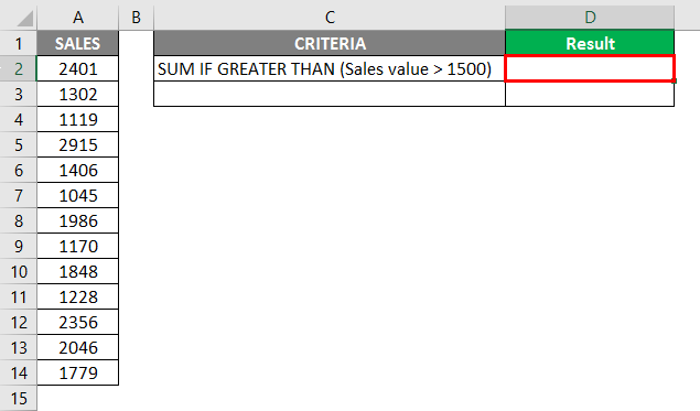
I have a sales value column A (A2 to A14) in the example below. So here, I want the sum of sales value which is greater than 1500, i.e., “>1500” from this sales dataset range (A2 to A14).
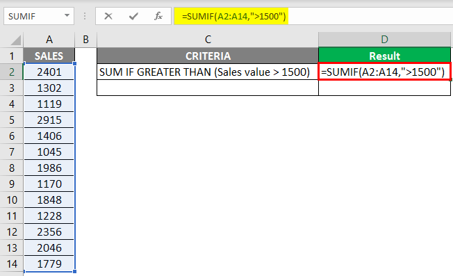
Now, let’s apply the SUMIF function in the cell “D2”, i.e., =SUMIF (range, criteria); you can skip the [sum_range] argument here.
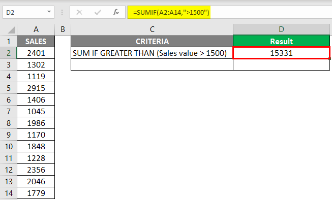
=SUMIF(A2: A14,”>1500″) formula sums the amounts in column D when they are greater than 1500 & returns the sum of sales value, i.e., 15331
b. SUMIF Function with Lesser Than (<) operator
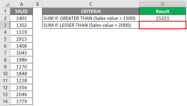
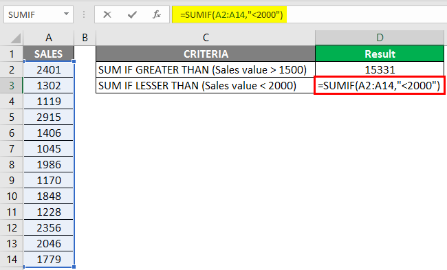
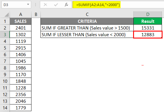
I have a sales value column I (A2 to A14) in the example below. So here, I want the sum of sales value which is lesser than 2000, i.e., “<2000” from this sales dataset range (A2 to A14).
Now, let’s apply the SUMIF function in the cell “D3”, i.e., =SUMIF (range, criteria); you can skip the [sum_range] argument here.
=SUMIF(A2: A14,” <2000″) formula sums the amounts in column D when they are lesser than 2000 & returns the sum of sales value, i.e., 15331
Example #3 – SUMIF Function with Wildcard Character
Suppose you want to sum up or add values for the cells containing specific text; wildcard characters will help you.
The most widely used wildcard characters in the Excel SUMIF function are:
(a) asterisk (*) To match any sequence of leading or trailing characters.
(b) Question mark (?) used to track, identify, or take a count of a single character.
SUMIF Function with Asterisk (*) Wildcard Character
SUMIF function supports wildcards like an asterisk (*) & Question mark (?). An asterisk (*) means “one or more characters.”
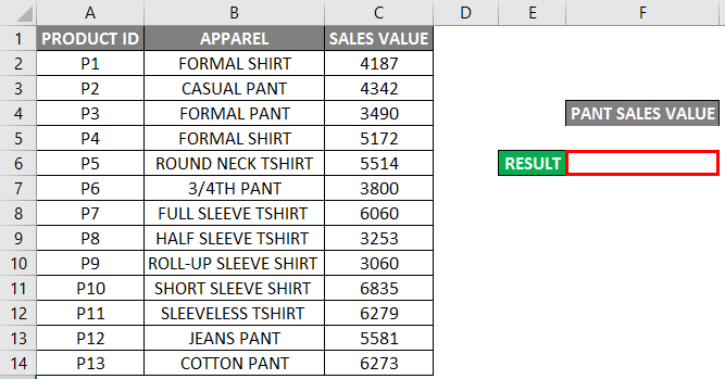
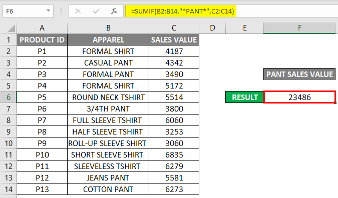
Suppose, in the below-mentioned example, I want to sum up OR add up the sales values for a specific text, i.e., the Apparel column containing “PANT” text in column C. Let’s check to use the SUMIF function with wildcard asterisk (*) in Excel.
In the below-mentioned example, the table contains the list of product IDs in column A (A2 to A14), apparel in column B (B2 to B14), and its sales value in column C (C2 to C14). Here I want the sum of sales value for the Apparel column containing “PANT” text.
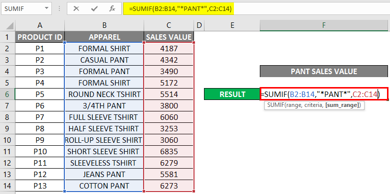
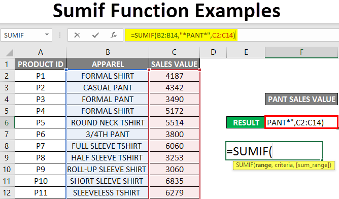
Let’s apply the SUMIF function in cell “F6″. I.E. =SUMIF (B2:B14,”*PANT*”,C2:C14)
The SUMIF function in the sums mentioned above OR adds up the range C2 to C14 if its corresponding or neighbor cells contain the keyword “PANT” in the range B2 to B14.
- Range: The range of cells needs to be evaluated by your criteria, i.e., column B. It is a range of cells containing the keyword “PANT”, i.e., B2 to B14.
- Criteria: Here, I want to match all apparel items that contain the keyword or specific text “PANT”; hence, the criteria are “*PANT*.”
- [sum_range]: Column C is an array or range of sales values that must be added. i.e. C2 to C14.
You can click enter after entering all three arguments in the SUMIF function.
=SUMIF (B2:B14,”*PANT*”,C2:C14)
i.e., returns the sum of sales value for the apparel “PANT”, i.e., “23486.”
Recommended Articles
This is a guide to Sumif Function Examples. Here we discuss How to use SUMIF Function in Excel, examples, and downloadable Excel templates. You may also look at these useful functions in Excel –

