Updated March 21, 2023
Introduction to NumPy Ndarray
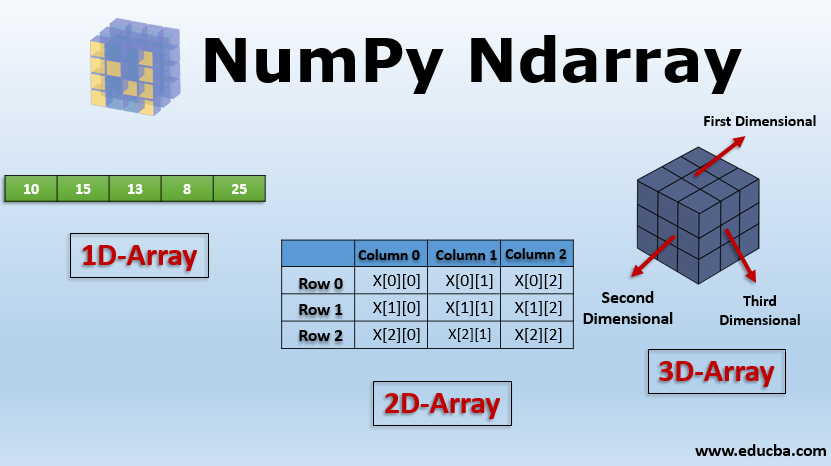
Ndarray is one of the most important classes in the NumPy python library. It is basically a multidimensional or n-dimensional array of fixed size with homogeneous elements( i.e., the data type of all the elements in the array is the same). A multidimensional array looks something like this:
In Numpy, the number of dimensions of the array is given by Rank. Thus, in the above example, the ranks of the array of 1D, 2D, and 3D arrays are 1, 2 and 3 respectively.
Syntax:
np.ndarray(shape, dtype= int, buffer=None, offset=0, strides=None, order=None)Here, the size and the number of elements present in the array is given by the shape attribute. The data type of the array(elements in particular) is given by the dtype attribute. Buffer attribute is an object exposing the buffer interface. An offset is the offset of the array data in the buffer. Stride attribute specifies the number of locations in the memory between the starting of successive array elements.
It should always be greater or equal to the size of the data type of the elements. Finally, the order attribute is to specify if we want a row-major or column-major order. Among all the above-mentioned attributes, shape and dtype are the compulsory ones. All other attributes are optional and can be specified on the requirement basis.
Working with Ndarray
An array can be created using the following functions :
- np.ndarray(shape, type): Creates an array of the given shape with random numbers.
- np.array(array_object): Creates an array of the given shape from the list or tuple.
- np.zeros(shape): Creates an array of the given shape with all zeros.
- np.ones(shape): Creates an array of the given shape with all ones.
- np.full(shape,array_object, dtype): Creates an array of the given shape with complex numbers.
- np.arange(range): Creates an array with the specified range.
Examples of Ndarray
Given below are the examples of Ndarray:
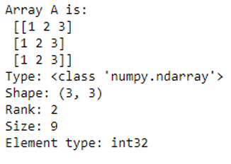
Example #1: Attributes of a multidimensional array(ndarray)
Code:
import numpy as np
#creating an array to understand its attributes
A = np.array([[1,2,3],[1,2,3],[1,2,3]])
print("Array A is:\n",A)
#type of array
print("Type:", type(A))
#Shape of array
print("Shape:", A.shape)
#no. of dimensions
print("Rank:", A.ndim)
#size of array
print("Size:", A.size)
#type of each element in the array
print("Element type:", A.dtype)
Output:
Example #2: Creation of a multidimensional array(ndarray)
Code:
import numpy as np
#creating array using ndarray
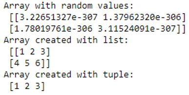
A = np.ndarray(shape=(2,2), dtype=float)
print("Array with random values:\n", A)
# Creating array from list
B = np.array([[1, 2, 3], [4, 5, 6]])
print ("Array created with list:\n", B)
# Creating array from tuple
C = np.array((1 , 2, 3))
print ("Array created with tuple:\n", C)
# Creating array with all ones
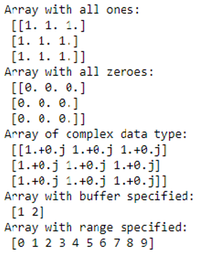
D = np.ones((3, 3))
print ("Array with all ones:\n", D)
# Creating array with all zeros
E = np.zeros((3, 3))
print ("Array with all zeroes:\n",E)
# Creating an array with complex data type
F = np.full((3, 3), 1, dtype = 'complex')
print ("Array of complex data type:\n", F)
#creating an array with buffer
G = np.ndarray((2,), buffer=np.array([1,2,3]),dtype=int)
print ("Array with buffer specified:\n", G)
#creating an array with range
H = np.arange(10)
print ("Array with range specified:\n", H)
Output:
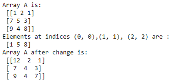
Example #3: Program to illustrate Indexing in 2D array
Code:
#creating an array to understand indexing
A = np.array([[1,2,1],[7,5,3],[9,4,8]])
print("Array A is:\n",A)
B = A[[0, 1, 2], [0, 1, 2]]
print ("Elements at indices (0, 0),(1, 1), (2, 2) are : \n",B)
#changing the value of elements at a given index
A[0,0] = 12
A[1,1] = 4
A[2,2] = 7
print("Array A after change is:\n", A)
Output:
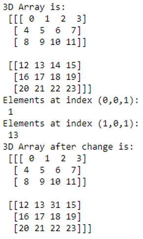
Example #4: Program to illustrate Indexing in a 3D array
Code:
#creating a 3d array to see indexing in a 3D array.
import numpy as np
I = np.array([[[ 0,  1,  2,  3],
[ 4,  5,  6,  7],
[ 8,  9, 10, 11]],
[[12, 13, 14, 15],
[16, 17, 18, 19],
[20, 21, 22, 23]]])
print("3D Array is:\n", I)
print("Elements at index (0,0,1):\n", I[0,0,1])
print("Elements at index (1,0,1):\n", I[1,0,1])
#changing the value of elements at a given index
I[1,0,2] = 31
print("3D Array after change is:\n", I)
Output:
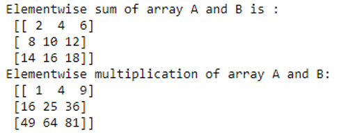
Example #5: Operations on Ndarray
Elementwise operations in Ndarrays.
Code:
import numpy as np
A = np.array([[1, 2, 3],
[4,5,6],[7,8,9]])
B = np.array([[1, 2, 3],
[4,5,6],[7,8,9]])
# adding arrays A and B
print ("Elementwise sum of array A and B is :\n", A + B)
# multiplying arrays A and B
print ("Elementwise multiplication of array A and B:\n", A*B)
Output:
Advantages of Ndarrays
- One of the main advantages of using Numpy Ndarrays is that they take less memory space and provide better runtime speed when compared with similar data structures in python(lists and tuples).
- Numpy Ndarrays support some specific scientific functions such as linear algebra. They help us in solving linear equations.
- Ndarrays support vectorized operations, like elementwise addition and multiplication, computing Kronecker product, etc. Python lists fail to support these features.
Conclusion – NumPy Ndarray
A NumPy Ndarray is a multidimensional array of objects all of the same type. It is immensely helpful in scientific and mathematical computing. As such, they find applications in data science, machine learning, and artificial intelligence. So, in order to be an efficient data scientist or machine learning engineer, one must be very comfortable with Numpy Ndarrays.
Recommended Articles
This has been a guide to NumPy Ndarray. Here we discuss the introduction, syntax, working, and various examples of NumPy Ndarray. You may also have a look at the following articles to learn more –

