Updated July 24, 2023
Deadweight Loss Formula (Table of Contents)
What is the Deadweight Loss Formula?
The term “deadweight loss” refers to the economic loss incurred due to inefficient market condition i.e. demand and supply are out of equilibrium.
In other words, deadweight loss indicates that the economic welfare of society is not at its optimum level. Some of the major causes of deadweight losses include rent control (price ceiling), minimum wage (price floor) and taxation.
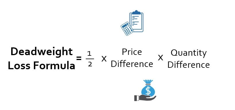
The formula for deadweight loss is expressed as the area of the triangle with base equivalent to the difference between prices of the original demand curve and new demand curve at the new quantity demanded and height equivalent to the difference between equilibrium quantities of the original demand curve and new demand curve. Mathematically, it is represented as,
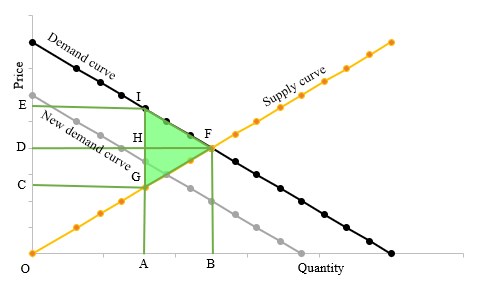
Geometrically, the formula for deadweight loss is expressed as the area of ΔIGF as illustrated in the graph shown below, which is bounded by the upward-sloping supply curve, the downward sloping demand curve and the vertical line drawn parallel to ordinate for price at a new equilibrium point.
In the above graph, a point I represents the price that the consumer was willing to pay initially (original demand curve) and G represents the price that the consumer is currently willing to pay (new demand curve). On the other hand, points B and A corresponds to the equilibrium quantities of the original and new demand curve respectively. Mathematically, the deadweight loss can be expressed as,
(Since AB || HF)
Examples of Deadweight Loss Formula (With Excel Template)
Let’s take an example to understand the calculation of Deadweight Loss in a better manner.
Deadweight Loss Formula – Example #1
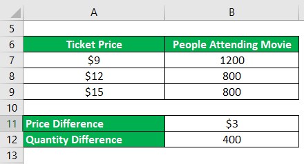
Let us take the example of demand and price of theatre tickets to illustrate the computation of deadweight loss. In a perfect market scenario, the theatre tickets are priced at $9 with 1,200 attending the movies. However, the government imposed a price floor of $12 due to which the demand declined to 800. In the perfect market scenario, 800 people would be attending the movies only of the price went upto $15. Calculate the movie theatre’s deadweight loss in the given scenario.
Solution:
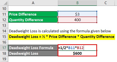
Deadweight Loss is calculated using the formula given below
Deadweight Loss = ½ * Price Difference * Quantity Difference
- Deadweight Loss = ½ * $3 * 400
- Deadweight Loss = $600
Therefore, the deadweight loss of the movie theatre, in this case, is equivalent to $600.
Deadweight Loss Formula – Example #2
Let us take another example wherein the original demand curve is represented by the equation (-0.08x + 80) and the supply curve by (0.08x), where ‘x’ is the quantity demand. However, due to some external factors, the demand curve shifted to (-0.08x + 60). Calculate the deadweight loss based on the given conditions.
Solution:
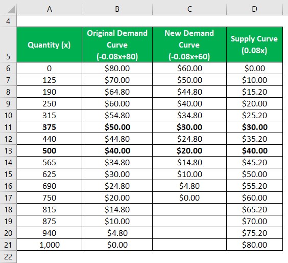
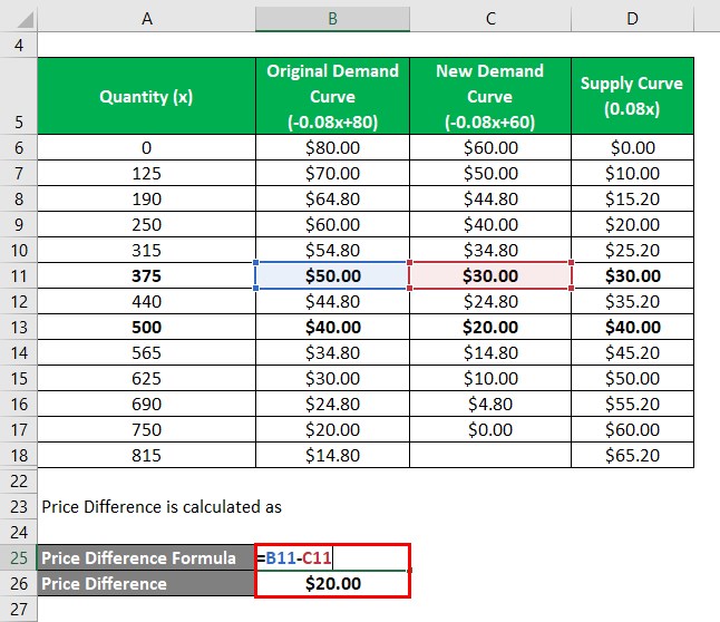
Now, let us build the table for the given original and new demand curves and the supply curve. For a detailed calculation of the same refer to section “Deadweight Loss Formula in Excel”.
- At zero demand price as per original demand curve = -0.08 * 0 +80 = $80
- At zero demand price as per new demand curve = -0.08 * 0 +60 = $60
- At zero demand price as per supply curve = 0.08 * 0 = $0
and so on so forth,
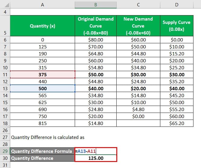
From the above table, it can be seen that the initial equilibrium quantity is 500 and the new equilibrium quantity is 375. On the other hand, the original price and new price at the new equilibrium are $50.00 and $30.00 respectively.
Therefore,
Price Difference is calculated as
- Price Difference = $50.00 – $30.00
- Price Difference = $20.00
Quantity Difference is calculated as
- Quantity Difference = 500 – 375
- Quantity Difference = 125.00
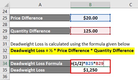
Deadweight Loss is calculated using the formula given below
Deadweight Loss = ½ * Price Difference * Quantity Difference
- Deadweight Loss = ½ * $20.00 * 125
- Deadweight Loss = $1,250
Explanation
The formula for deadweight loss can be derived by using the following steps:
Step 1: Firstly, plot graph for the supply curve and the initial demand curve with a price on the ordinate and quantity on the abscissa. Then, determine the equilibrium quantity, where the demand curve meets the supply curve. In the graph, the equilibrium point is denoted by F and the quantity by OB.
Step 2: Next, draw the line for the new demand curve which is the actual demand scenario which is out of equilibrium. Then, determine the equilibrium quantity at this current demand level. In the graph, the point is denoted by G and the quantity is denoted by OA.
Step 3: Next, draw a line parallel to the ordinate and passing through new equilibrium quantity G such that it intersects the original demand curve at I. Then, determine the price that the consumer would have paid for the original demand level and what it will actually now. The price point on the original demand curve is I and the new demand curve is G, while the prices are OE and OC respectively.
Step 4: Next, compute the difference between the original and new equilibrium quantity.
Quantity Difference = OB – OA = AB
Which is parallel to HF.
Step 5: Next, compute the difference between the prices paid for the original and new demand curve at the new equilibrium quantity.
Price Difference = OE – OC = EC
Which is parallel to IG.
Step 6: Finally, the formula for deadweight loss is expressed as the area of the triangle with base equivalent to price difference (step 5) and height equivalent to quantity difference (step 4) as shown below.
Deadweight Loss = ½ * Price Difference * Quantity Difference
or
Deadweight Loss = ½ * IG * HF
Relevance and Use of Deadweight Loss Formula
The concept of deadweight loss is important from an economic point of view as it helps is the assessment of the welfare of society. Basically, it is a measure of the inefficiency of a market, such that a higher value of deadweight loss indicates a greater degree of inefficiency prevalent in the market. Such losses are witnessed in the market characterized by oligopoly and monopoly.
Deadweight Loss Formula Calculator
You can use the following Deadweight Loss Formula Calculator
| Price Difference | |
| Quantity Difference | |
| Deadweight Loss | |
| Deadweight Loss = ½ * | Price Difference * Quantity Difference |
| ½ *0 *0 = 0 |
Recommended Articles
This is a guide to the Deadweight Loss Formula. Here we discuss how to calculate deadweight loss along with practical examples. we also provide a deadweight loss calculator with a downloadable excel template. You may also look at the following articles to learn more –
