Updated June 8, 2023
Introduction to Autofit Row Height
All of us know that by default, all the rows in Excel are set to some unique height, which is 15 points, which equals 20 pixels. However, we can change the row height as per our requirement and also be autofitted to apply the height of one row to all other rows. This is something that Excel has as an added benefit and usually works in the favor of users like us. We can change the row height using different techniques in Excel. You can use a mouse to change the row height, or you can change it using Format, which is placed within Cells Group under the Home tab, or you can use AutoFit Row Height option, or maybe Wrap Text can come in to help you change the row height. However, within all these varieties of options, Autofit Row Height has a beauty of its own. This article provides insight into Autofit Row Height in Excel.
What is Excel AutoFit Row Height?
Well, we all know that row height is dependent on font size. Decreasing or increasing the font size for a row changes its height accordingly (directly proportional to font size). There are times when you copy the data from a different source and paste it with source formatting, which causes the text to be clipped under the row as shown below:
If there are few lines, you can adjust the row height manually with the help of different options, which we already discussed in the introduction part of this article. However, think of a situation where you have huge data possibly spread across rows numbered in millions. It will be difficult to change the row height in that case manually. Therefore, we have AutoFit Row Height utility in Excel that allows the row to expand automatically depending on the font size of the largest value in the row.
Examples of AutoFit Row Height in Excel
Let’s discuss the examples of AutoFit Row Height in Excel.
Example #1 – How to Change Row Height?
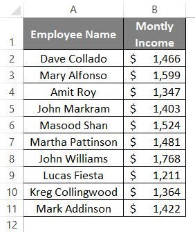
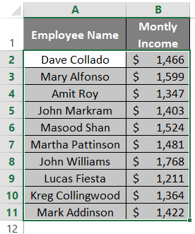
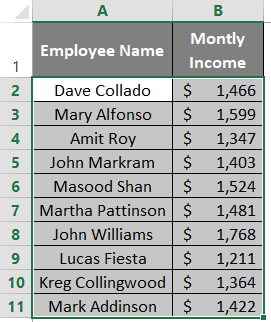
The first thing we’ll look into in this article is how to change the row height for a specific group of cells. You can change row height by dragging the row border upwards or downwards to increase or decrease height respectively. Once the row height is changed, you can use the Format Painter tool from Excel to apply the same formatting across different rows. Suppose we have data as shown below. This data specifies the Employee Names and the Monthly Income for the same:
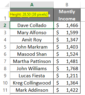
Step 1: I will try to change the height of the second row and set it for 21 points. Put your mouse cursor to the end of the second-row border and drag it down until the height becomes 21 points. You’ll see the height values while you drag the border down.
Now, we would like to apply the same row height for other cells of this Excel book. This task is easy with the help of the Format Painter utility in Excel.
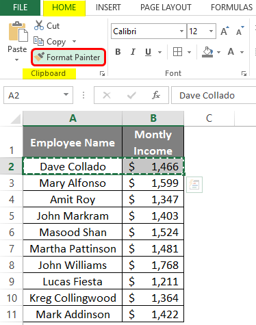
Step 2: Select the entire second row for which we just have changed the row height to 21 points and click on the Format Painter option within the Clipboard group under the Home tab.
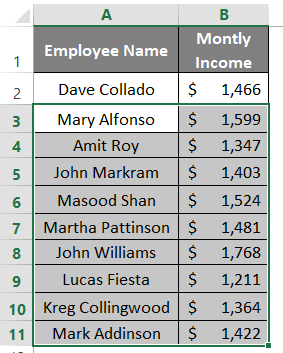
Step 3: Use the Format Painter brushes to apply the copied format to all other rows where you wish the row height to be the same as the first row.
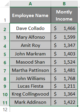
All the rows (which have data; spreading across A2:B11) are now the same height as that of 21 points. This is how we can change the row heights to our needs.
Example #2 – AutoFit Row Height in Excel
We will now see how to use Excel’s AutoFit Row Height utility to automatically fit the row height to the best fit. As discussed earlier, this utility is based on the text size present in a particular row. There are two ways of auto-adjusting the row height in Excel.
Method#1 – Auto Adjust Row Height in Excel
Step 1: Select all the rows you wanted to autofit the row height based on the text size within cells. In this case, I will select all rows from the second to the eleventh row.
Make sure you select the entire row and not only the cells where data is present. If done so, you’ll be unable to autofit the row height.
Step 2: Now, go to any of the row borders and place your mouse cursor there. WYou’llhen you place the cursor on the row border, you’ll see a drag down sign.
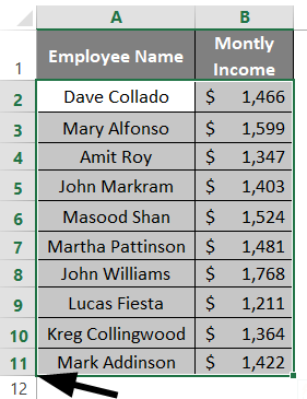
Step 3: Place the cursor on the last row boundary, double click the row border, and you’ll see row heights adjusted to the text size throughout the second to the eleventh row.
Method #2 – Auto Adjust the Row Height in Excel
Let’s see another method that allows us to auto adjust the row height in Excel. Follow the steps below:
Step 1: Select all the row height rows you want to change.
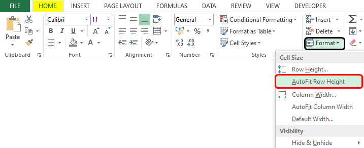
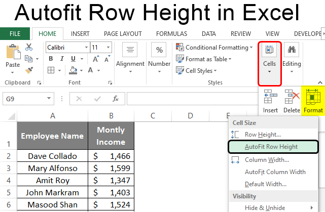
Step 2: Click on the Home tab, and navigate towards the Cells group, within which you can see the Format dropdown as shown below:
Step 3: Click on the Format dropdown under the Cells group to see the AutoFit Row Height option. Click on it.
When you click on the AutoFit Row Height option under Format, you can see the row heights for selected rows are auto-adjusted to the text size within the cells.
This is how AutoFit Row Height in Excel works. This article ends here. Let’s wrap things up with some points to be remembered.
Things to Remember
- The default row height in Excel is 15 points which is equal to 20 pixels.
- Ideally, the height of rows in Excel depends on the font size of the text present in any row cell, and it is directly proportional to the row height. This means a sufficient increase in font size increases the row height and vice-versa.
- You can also use Alt + O + R + A as a keyboard shortcut to automatically adjust the row height based on the font size of the text present in any cell of the row/s.
Recommended Articles
This has been a guide to Autofit Row Height in Excel. Here we discuss How to change Autofit Row Height in Excel, practical examples, and a downloadable Excel template. You can also go through our other suggested articles –

