Introduction to Curve Fitting Matlab
The Curve Fitting module is used for graphical user interfaces (GUIs) and M-file entities. It built on the MATLAB technical computing environment. The toolbox provides you feature like Data pre-processing such as sectioning and smoothing. A graphical environment (GUIs) that allows you to explore and analyze data sets and fits visually and numerically and also save your work in various formats including M-files as well as binary files and workspace variables. In this topic, we are going to learn about Curve Fitting Matlab.
Syntax
q= polyfit ( a,y,n)

[q,S] = polyfit(a,y,n)

[q,S,u] = polyfit (a,y,n)
Description
q = polyfit(a,y,n) returns the coefficients for a polynomial q(a) of degree n that is the best fit (in a least-squares sense) for the data in y. The coefficients in q are in descending powers, and the length of q is n+1.
[q,S] = polyfit(a,y,n) also returns a structure S they can be used as an input to the polyval to obtain error estimates. [q,S,u] = polyfit(a,y,n) also returns u and in which here a two-element vector with centering and scaling values. U (1) is mean(a), and u(2) is std(a). Using these values, polyfitcentrea at zero and scales it to have a unit standard deviationThe Curve Fitting Matlab toolbox provides a one-term and a two-term exponential model. The exponential curve is obtained when the rate of change of a quantity is proportional to the initial amount of the quantity. If the coefficient associated with an ax and/or yz is negative, q represents exponential decay. If the coefficient is positive, q represents exponential growth.
Examples of Curve Fitting Matlab
Here are the following examples mention below:
Example #1
Consider the example of a polynomial curve in which we can see how to use polynomial entities in the form of the curve. variable = polyfit(var1,var2,n),Where var1 and var2 are co-ordinates of two vectors
Code:
ax = [1 2 3 4 4.9];

y = [5.5 43.1 128 290.7 498.4];

p = polyfit(ax,y,3)

x2 = 1:.1:5;

y2 = polyval(p,x2);

plot(ax,y,'o',x2,y2)

grid on

s = sprintf('y = (%.1f) x^3 + (%.1f) x^2 + (%.1f) x + (%.1f)',p(1),p(2),p(3),p(4));

text(2,400,s)
Output:
Example #2
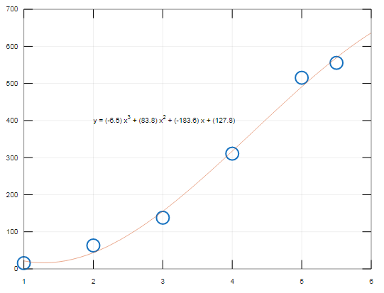
Consider 2nd` no. example of a polynomial curve, in which the polyfit syntax is used.
In the below example 6 points curve is shown .in which how to draw the polynomial curve is shown in a simple manner using polyfit syntax. Also the Output is given below the program.
Code:
ax = [1 2 3 4 5 5.5];

y = [15.5 63.1 138 310.7 515.4 555.56];

p = polyfit(ax,y,3)

x2 = 1:.1:6;

y2 = polyval(p,x2);

plot(ax,y,'o',x2,y2)

grid on

s = sprintf('y = (%.1f) x^3 + (%.1f) x^2 + (%.1f) x + (%.1f)',p(1),p(2),p(3),p(4));

text(2,400,s)
Output:
Example #3
Consider 3rd` no. example of the polynomial curve, in which the polyfit syntax is used
Also. Polyval Matlab in build function is used
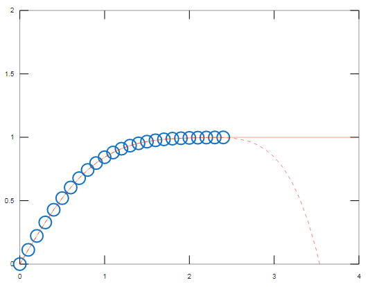
In the below example, the exponential curve is shown .in which how to draw the polynomial curve is shown in a simple manner using polyfit syntax. Also the Output is given below the program.
Code:
ax = (0:0.1:2.4)';

yz = erf(ax);

p = polyfit(ax,yz,5);

f = polyval(p,ax);

T = table(ax,yz,f,yz-f,'VariableNames',{'X','Y','Fit','FitError'});

x1 = (0:0.1:5)';

y1 = erf(x1);

f1 = polyval(p,x1);

figure

plot(ax,yz,'o')

hold on

plot(x1,y1,'-')

plot(x1,f1,'r--')

axis([0  4  0  2])

hold off
Output:
Conclusion
In this article we have seen how to use Curve fitting, also known as regression analysis, Curve fitting is used to find the “best fit” line or curve for a series of data points. curve fitting mostly creates an equation that is used to find coordinates along the path, you may not be concerned about finding an equation.
Recommended Articles
This is a guide to Curve Fitting Matlab. Here we discuss how to use Curve fitting in Matlab with respective programming examples for understanding better. You may also have a look at the following articles to learn more –


