Updated March 3, 2023
Introduction to Varargin in Matlab
MATLAB is a programming environment that is interactive and is used in scientific computing. It is extensively used in a lot of technical fields where problem-solving, data analysis, algorithm development, and experimentation is required. The software which are discipline-specific is extensively written using MATLAB.
In this article, we will study how to use ‘varargin’ input variable in MATLAB.
Before we start learning how ‘varargin’ works in MATLAB, let us understand why we need ‘varargin’ input variable.
VARARGIN
We use ‘varargin’ inside definition of a function so that we can pass as many arguments as we need. In some situations, it becomes difficult for a coder to decide the number of input arguments upfront. These situations require a function definition to be flexible enough to accept any number of arguments while calling it.
Let us now understand the syntax of ‘varargin’ in MATLAB:
Syntax:
varargin
[Please keep in mind that ‘varargin’ is in lowercase and passed as the last argument to the function]
Description:
- varargin is passed as an input variable to a function definition
- It provides the function with the ability to accept as many arguments as the coder wants.
Examples of Varargin in Matlab
Let us now understand how the code for ‘varargin’ looks like in MATLAB, with the help of various examples.
Example #1
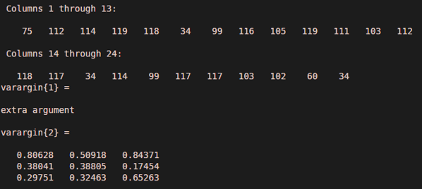
In this example, we will define a function that will simply display the number of arguments passed. We will need to follow the following 2 steps:
- Create a file with a function stored in it. This will have ‘.m’ extension
- Call the function created in the above file
Code to create the function and save it as .m extension:
function learningVarargin (varargin)
[Defining the function learningVarargin and passing the ‘varargin’ command]
disp ("Input arguments passed: " + nargin)
[‘nargin’ is used to get the number of input variables]
celldisp (varargin)
[‘celldisp’ will display all the input variables]
end
[After creating the function, save this file by the name of your choice, here we are naming our file as ‘learningVarargin.m]
Now in the new command window, use the following code:
Code to call the function
type learningVarargin

learningVarargin ('extra argument', rand (3))
[Calling the learningVarargin function using arguments of our choice. Here we have used 2 arguments to call the function]
Input 1 (Creating the function):
function learningVarargin (varargin)

disp ("Input arguments passed: " + nargin)

celldisp (varargin)

end
Input 2 (Calling the function):
type learningVarargin

learningVarargin ('extra argument', rand (3))
Output:
Example #2
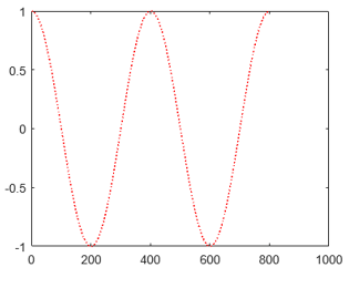
In this example, we will define a function that will plot a cos wave. We will pass the number of arguments to format the style of a plot as per or requirement.
Code to create the function and save it as .m extension:
function learningVarargin1 (x, varargin)
[Defining the function learningVarargin1 and passing the ‘varargin’ command]
plot (x, varargin {:})
[plot is used to get the graph]
varargin {:} will help us to pass as many arguments as we want to the plot]
end
[After creating the function, save this file by the name of your choice, here we are naming our file as ‘learningVarargin1.m]
Code to call the function
type learningVarargin1

learningVarargin1 (cos (0 : pi/200 : 4*pi), 'color', 'r', 'linestyle', ':')
[Calling the learningVarargin1 function using arguments of our choice. Here we have used ‘color’ and ‘linestyle’ argument in addition to the mandatory argument ‘x’, to call the function]
Input 1 (Creating the function):
function learningVarargin1 (x, varargin)

plot (x, varargin {:})

end
Input 2 (Calling the function):
type learningVarargin1

learningVarargin1 (cos (0 : pi/200 : 4*pi), 'color', 'r', 'linestyle', ':')
Output:
Example #3
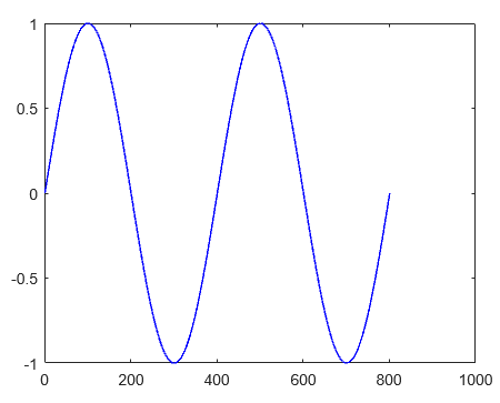
In this example, we will define a function which will plot a sine wave. We will pass different arguments from the ones passed above, to format the style of plot.
Code to create the function and save it as .m extension:
function learningVarargin2 (x, varargin)
[Defining the function learningVarargin2 and passing the ‘varargin’ command]
[Here, notice that the syntax for the function remains essentially the same. This is the power of ‘varargin’ command which will help us change the number of input arguments while calling the function, without worrying about the number of arguments]
Code to call the function
type learningVarargin2

learningVarargin1 (sine (0 : pi/200 : 4*pi), 'color', 'r')
[Calling the learningVarargin2 function using arguments of our choice. Here we have used only color argument in addition to the mandatory argument ‘x’, to call the function]
Input 1 (Creating the function):
function learningVarargin2 (x, varargin)

plot (x, varargin {:})

end
Input 2 (Calling the function):
type learningVarargin2

learningVarargin1 (sine (0 : pi/200 : 4*pi), 'color', 'b')
Output:
Conclusion
‘varargin’ can be used in MATLAB when we are not sure how many arguments we might need while calling the function. The flexibility it offers becomes very useful when using functions like plot, where we might need to format the graph on the go.
Recommended Articles
This is a guide to Varargin in Matlab. Here we discuss Introduction, syntax, Description, and Examples with code implementation. You can also go through our other related articles to learn more –


