Definition of Data Imputation
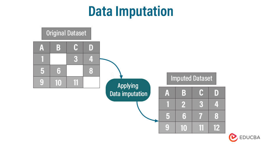
Data imputation is the process of replacing missing or incomplete data points in a dataset with estimated or substituted values. These estimated values are typically derived from the available data, statistical methods, or machine learning algorithms.
Data imputation fills missing values in datasets, preserving data completeness and quality. It ensures practical analysis, model performance, and visualizations by preventing data loss and maintaining sample size. Imputation reduces bias, maintains data relationships, and facilitates various statistical techniques, enabling better decision-making and insights from incomplete data.
Table of Contents
- Definition
- Importance
- Techniques
- Mean/Median/Mode Imputation
- Forward Fill and Backward Fill
- Linear Regression Imputation
- Interpolation and Extrapolation
- K-Nearest Neighbors (KNN) Imputation
- Expectation-maximization (EM) Imputation
- Regression Trees and Random Forests
- Deep Learning-Based Imputation
- Hot Deck Imputation
- Time Series Imputation
- Manual Imputation
- Types of Missing Data
- Best Practices
- Multiple Imputation vs Missing Imputation
- Potential Challenges
- Future Developments
Importance of Data Imputation in Analysis
Data imputation is crucial in data analysis as it addresses missing or incomplete data, ensuring the integrity of analyses. Imputed data enables the use of various statistical methods and machine learning algorithms, improving model accuracy and predictive power. Without imputation, valuable information may be lost, leading to biased or less reliable results. It helps maintain sample size, reduces bias, and enhances the overall quality and reliability of data-driven insights.
Data Imputation Techniques
There are several methods and techniques for data imputation, each with its strengths and suitability depending on the nature of the data and the analysis goals. Let’s discuss some commonly used data imputation techniques:
1. Mean/Median/Mode Imputation
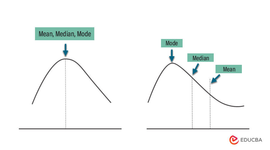
- Mean Imputation: Replace missing values in numerical variables with the average of the observed values for that variable.
- Median Imputation: Replace missing values in numerical variables with the middle value of the observed values for that variable.
- Mode Imputation: Replace missing values in categorical variables with the most frequent category among the observed values for that variable.
Steps:
- Identify variables with missing values.
- Compute the mean, median, or mode of the variable, depending on the chosen imputation method.
- Replace missing values in the variable with the computed central tendency measure.
| Advantages | Disadvantages and Considerations |
| Simplicity | Ignores Data Relationships |
| Preserves Data Structure | May Distort Data |
| Applicability | Inappropriate for Missing Data Patterns |
When to Use:
- Use mean imputation for numerical variables when missing data is missing completely at random (MCAR) and the variable has a relatively normal distribution.
- Use median imputation when the data is skewed or contains outliers, as it is less sensitive to extreme values.
- Use mode imputation for categorical variables when you have missing values that can be reasonably replaced with the most frequent category.
2. Forward Fill and Backward Fill
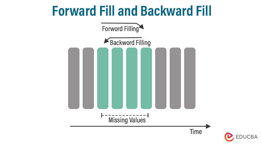
- Forward Fill: In forward fill imputation, missing values are replaced with the most recent observed value in the sequence. It propagates the last known value forward until a new observation is encountered.
- Backward Fill: In backward fill imputation, missing values are replaced with the next observed value in the sequence. It propagates the next known value backward until a new observation is encountered.
Steps:
- Identify the variables with missing values in a time-ordered dataset.
- For forward fill, replace each missing value with the most recent observed value that precedes it in time.
- For backward fill, replace each missing value with the next observed value that follows it in time.
| Advantages | Disadvantages and Considerations |
| Temporal Context | Assumption of Temporal Continuity |
| Simplicity | Potential Bias |
| Applicability | Missing Data Patterns |
When to Use:
- Use forward fill when you believe that missing values can be reasonably approximated by the most recent preceding value and you want to maintain the temporal context.
- Use backward fill when you believe that missing values can be reasonably approximated by the next available value and you want to maintain the temporal context.
3. Linear Regression Imputation
Linear regression imputation is a statistical imputation technique that leverages linear regression models to predict missing values based on the relationships observed between the variable with missing data and other relevant variables in the dataset.
Steps:
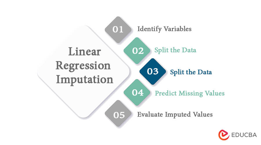
- Identify Variables: Determine the variable with missing values (the dependent variable) and the predictor variables (independent variables) that will be used to predict the missing values.
- Split the Data: Split the dataset into two subsets: one with complete data for the dependent and predictor variables and another with missing values for the dependent variable.
- Build a Linear Regression Model: Use the subset with complete data to build a linear regression model.
- Predict Missing Values: Apply the trained linear regression model to the subset with missing values to predict and fill in the missing values for the dependent variable.
- Evaluate Imputed Values: Assess the quality of the imputed values by examining their distribution, checking for outliers, and comparing them to observed values where available.
| Advantages | Disadvantages and Considerations |
| Utilizes Relationships | Assumption of Linearity |
| Predictive Accuracy | Sensitivity to Outliers |
| Preserves Data Structure | Model Selection |
When to Use:
When there is a known or plausible linear relationship between the variable with missing values and other variables in the dataset and the dataset is sufficiently large to build a robust linear regression model.
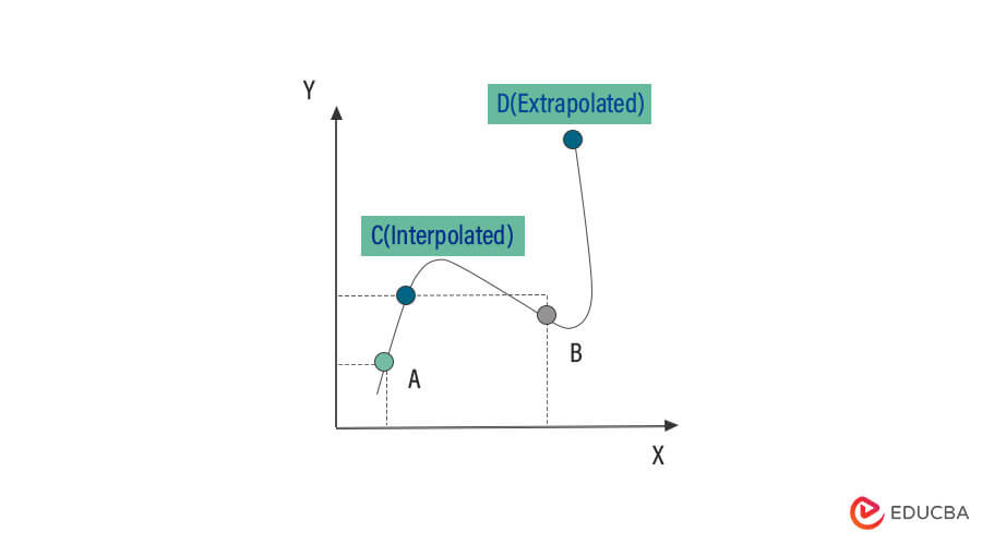
4. Interpolation and Extrapolation
Interpolation
Interpolation is the process of estimating values between two or more known data points.
Steps:
- Identify or collect a set of data points.
- Choose an interpolation method based on the nature of the data (e.g., linear, polynomial, spline).
- Apply the chosen method to estimate values within the data range.
| Advantages | Disadvantages and Considerations |
| Provide reasonable estimates within the range of observed data. | Assumes a continuous relationship between data points, which may not always hold. |
| Useful for filling gaps in data or estimating missing values. | Accuracy decreases as you move further from the known data points. |
Extrapolation
Extrapolation is the process of estimating values beyond the range of known data points.
Steps:
- Identify or collect a set of data points.
- Determine the nature of the data trend (e.g., linear, exponential, logarithmic).
- Extend the trend beyond the range of observed data to make predictions.
| Advantages | Disadvantages and Considerations |
| Allows for making predictions or projections into the future or past. | Extrapolation assumes that the data trend continues, which may not always be accurate. |
| Useful for forecasting and trend analysis. | Extrapolation can lead to significant errors if the underlying data pattern changes. |
When to Use:
- Interpolation is suitable when you have a series of data points and want to estimate values within the observed data range.
- Extrapolation is appropriate when you have historical data and want to make predictions or forecasts beyond the observed data range.
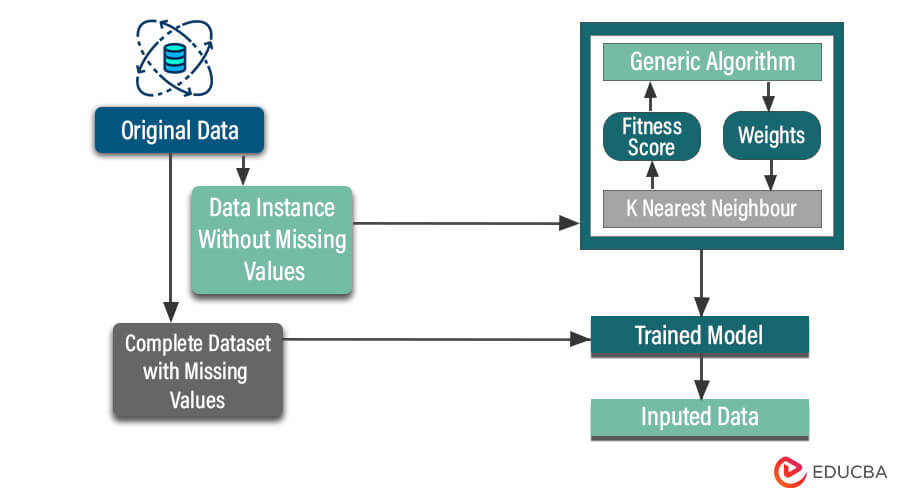
5. K-Nearest Neighbors (KNN) Imputation
K-nearest neighbors (KNN) Imputation is a method for handling missing data by estimating missing values using the values of their K-nearest neighbors, which are determined based on a similarity metric (e.g., Euclidean distance or cosine similarity) in the feature space.
Steps in KNN Imputation:
- Data Preprocessing: Prepare the dataset by identifying the variable(s) with missing values and selecting relevant features for similarity measurement.
- Normalization or Standardization: Normalize or standardize the dataset to ensure that variables are on the same scale, as distance-based methods like KNN are sensitive to scale differences.
- Distance Computation: Calculate the distance (similarity) between data points, typically using a distance metric such as Euclidean distance, Manhattan distance, or cosine similarity.
- Nearest Neighbors Selection: Identify the K-nearest neighbors for each data point with missing values based on the computed distances.
- Imputation: Calculate the imputed value for each missing data point as a weighted average (for continuous data) or a majority vote (for categorical data) of the values from its K-nearest neighbors.
- Repeat for All Missing Values: Repeat the above steps for all data points with missing values, imputing each missing value separately.
| Advantages | Disadvantages and Considerations |
| Utilizes information from similar data points to estimate missing values. | Sensitive to distance metric selection and a number of neighbors (K). |
| Can capture complex relationships in the data when K is appropriately chosen. | The effectiveness of KNN imputation depends on the assumption that similar data points have similar values, which may not hold in all cases. |
When to Use:
When you have a dataset with missing values and believe that similar data points are likely to have similar values, you need to impute missing values in both continuous and categorical variables.
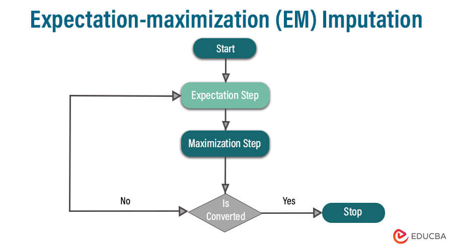
6. Expectation-maximization (EM) Imputation
Expectation-maximization (EM) imputation is an iterative statistical method for handling missing data.
Steps:
- Model Specification: Define a probabilistic model that represents the relationship between observed and missing data.
- Initialization: Start with an initial guess of the model parameters and imputed values for missing data. Common initializations include imputing missing values with their mean or using another imputation method.
- Expectation (E-step): In this step, calculate the expected values of the missing data (conditional on the observed data) using the current model parameters.
- Maximization (M-step): Update the model parameters to maximize the likelihood of the observed data, given the expected values from the E-step. This involves finding parameter estimates that make the observed data most probable.
- Iterate: Repeat the E-step and M-step until convergence is achieved. Convergence is typically determined by monitoring changes in the model parameters or log-likelihood between iterations.
- Imputation: Once the EM algorithm converges, use the final model parameters to impute the missing values in the dataset.
| Advantages | Disadvantages and Considerations |
| Can handle missing data that is not missing completely at random (i.e., data with a missing data mechanism) | Sensitivity to model misspecification: If the model is not a good fit for the data, imputed values may be biased. |
| Utilizes the underlying statistical structure in the data to make imputations, potentially leading to more accurate estimates. | Computationally intensive: EM imputation can be computationally expensive, especially for large datasets or complex models. |
When to Use:
- When you have a dataset with missing data, and you suspect that the missing data mechanism is not completely random.
- When there is an underlying statistical model that can describe the relationship between observed and missing data.
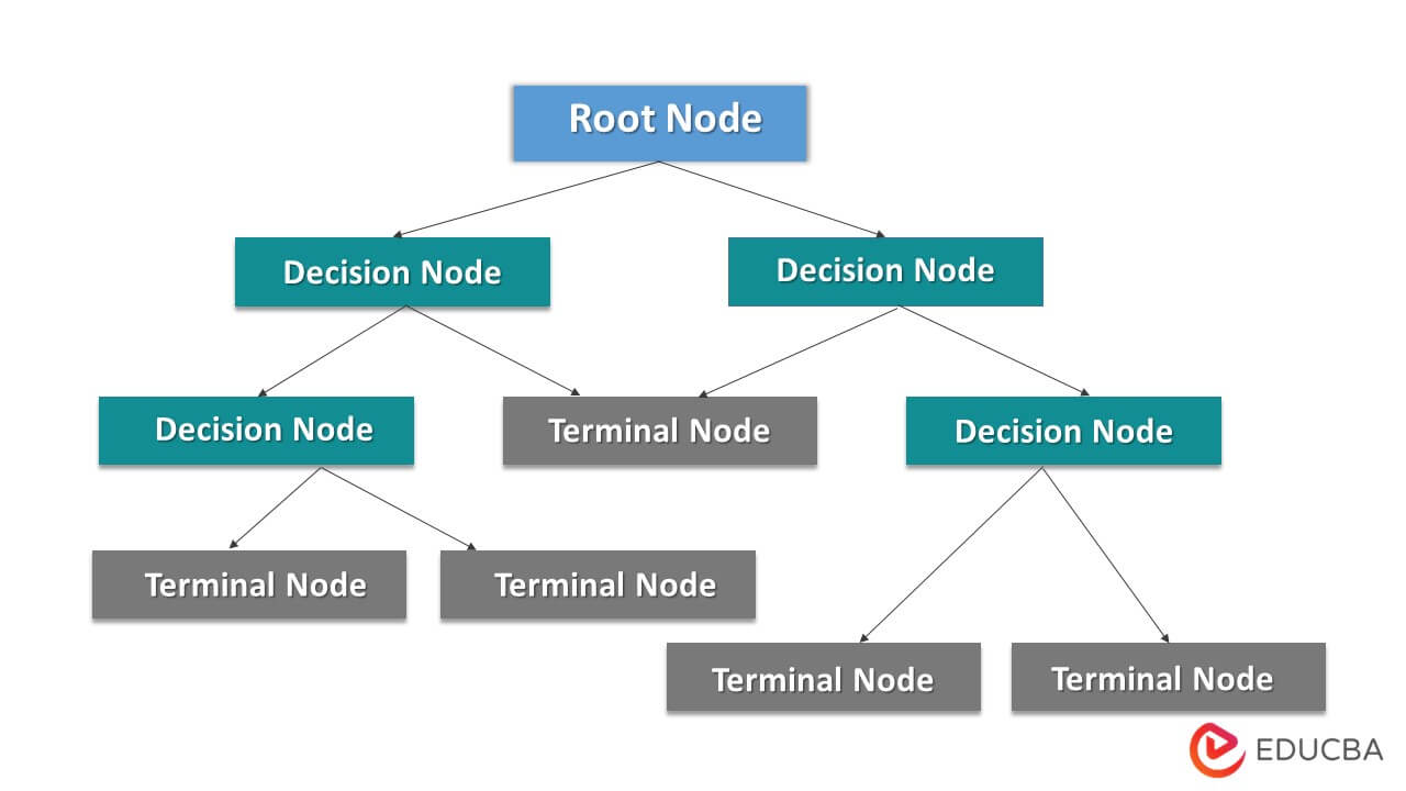
7. Regression Trees and Random Forests
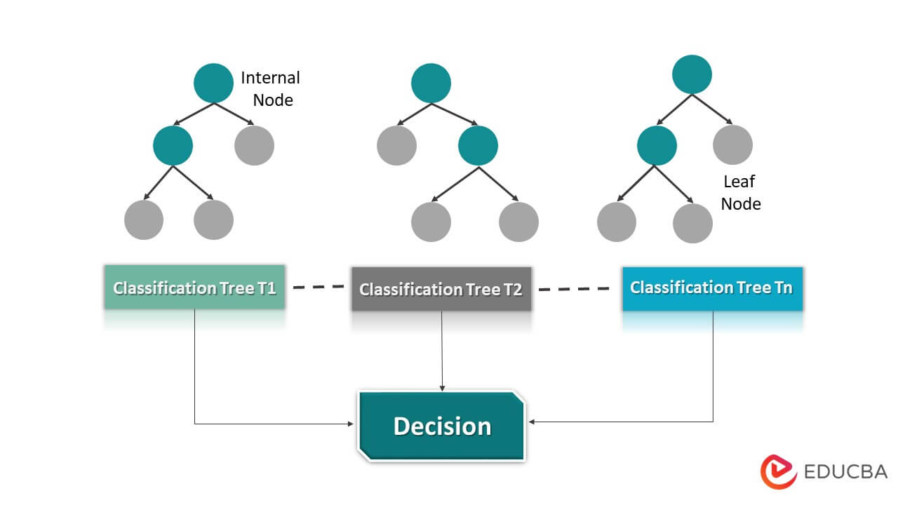
Regression Trees and Random Forests are machine-learning techniques used primarily for regression tasks. They are both based on decision tree algorithms but differ in their complexity and ability to handle complex data.
Regression Trees
Regression trees are a type of decision tree used for regression analysis. They divide the dataset into subsets, called leaves or terminal nodes, based on the input features and assign a constant value (usually the mean or median) to each leaf.
Steps:
- Start with the entire dataset.
- Select a feature and a split point that best divides the data based on a criterion (e.g., mean squared error).
- Repeat the splitting process for each branch until a stopping criterion is met (e.g., maximum depth or minimum number of samples per leaf).
- Assign a constant value to each leaf, typically the mean or median of the target variable.
| Advantages | Disadvantages and Considerations |
| Easy to interpret and visualize. | Prone to overfitting, especially when the tree is deep. |
| Handles both numerical and categorical data. | Sensitive to small variations in the data. |
| Can capture non-linear relationships. | Single trees may not generalize well to new data. |
Random Forests
Random Forests are an ensemble learning technique that consists of multiple decision trees, typically built using the bagging (bootstrap aggregating) method.
Steps:
- Randomly select subsets of the data (bootstrapping) and features (feature bagging) for each tree.
- Build individual decision trees for each subset.
- Combine the predictions of all trees (e.g., by averaging for regression) to make the final prediction.
| Advantages | Disadvantages and Considerations |
| Reduces overfitting by combining multiple models. | Can be computationally expensive for a large number of trees and features. |
| Provides feature importance scores. | The resulting model is less interpretable compared to a single decision tree |
When to Use:
- Use a single regression tree when you want a simple, interpretable model and have a small to moderate-sized dataset.
- Use Random Forests when you need high predictive accuracy, want to reduce overfitting, and have a larger dataset.
8. Deep Learning-Based Imputation
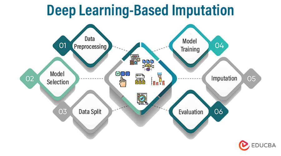
Deep Learning-Based Imputation is a data imputation method that uses deep neural networks to predict and fill in missing values in a dataset.
Steps:
- Data Preprocessing: Prepare the dataset by identifying the variable(s) with missing values and normalizing or standardizing the data as needed.
- Model Selection: Choose an appropriate deep-learning architecture for imputation. Common choices include feedforward neural networks and recurrent neural networks (RNNs).
- Data Split: Split the dataset into two parts: one with complete data (used for training) and another with missing values (used for imputation).
- Model Training: Train the selected deep learning model using the portion of the dataset with complete data as input and the same data as output (supervised training).
- Imputation: Use the trained model to predict missing values in the dataset with missing data based on the available information.
- Evaluation: Assess the quality of the imputed values by comparing them to observed values where available. Common evaluation metrics include mean squared error (MSE) or mean absolute error (MAE).
| Advantages | Disadvantages and Considerations |
| Ability to capture complex relationships | Computational complexity |
| Data-driven imputations. | Data requirements |
| High performance. | Interpretability |
When to Use:
- When dealing with large and complex datasets where traditional imputation methods may not be effective.
- When you have access to substantial computing resources for model training.
- when you prioritize predictive accuracy over interpretability.
Deep learning-based imputation may not be necessary for smaller, simpler datasets where simpler methods can suffice.
9. Hot Deck Imputation
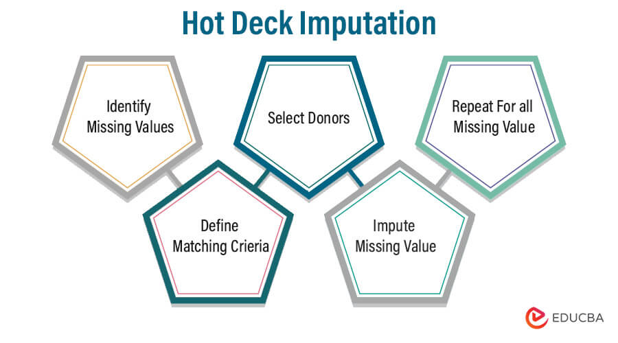
Hot Deck Imputation is a non-statistical imputation method that replaces missing values with observed values from similar or matching cases (donors) within the same dataset.
Steps:
- Identify Missing Values: Determine which variables in your dataset have missing values that need to be imputed.
- Define Matching Criteria: Specify the criteria for identifying similar or matching cases.
- Select Donors: For each record with missing data, search for matching cases (donors) within the dataset based on the defined criteria.
- Impute Missing Values: Replace the missing values in the target variable with values from the selected donor(s).
- Repeat for All Missing Values: Continue the process for all records with missing data until all missing values are imputed.
| Advantages | Disadvantages and Considerations |
| Maintains dataset structure | Assumes similarity |
| Simplicity | Limited to existing data |
| Can be useful for small datasets or when computational resources are limited. | Potential for bias |
When to Use:
When you have
- a small to moderately sized dataset and limited computational resources.
- want to maintain the existing relationships and structure within the dataset.
- you have reason to believe that similar cases should have similar values for the variable with missing data.
10. Time Series Imputation
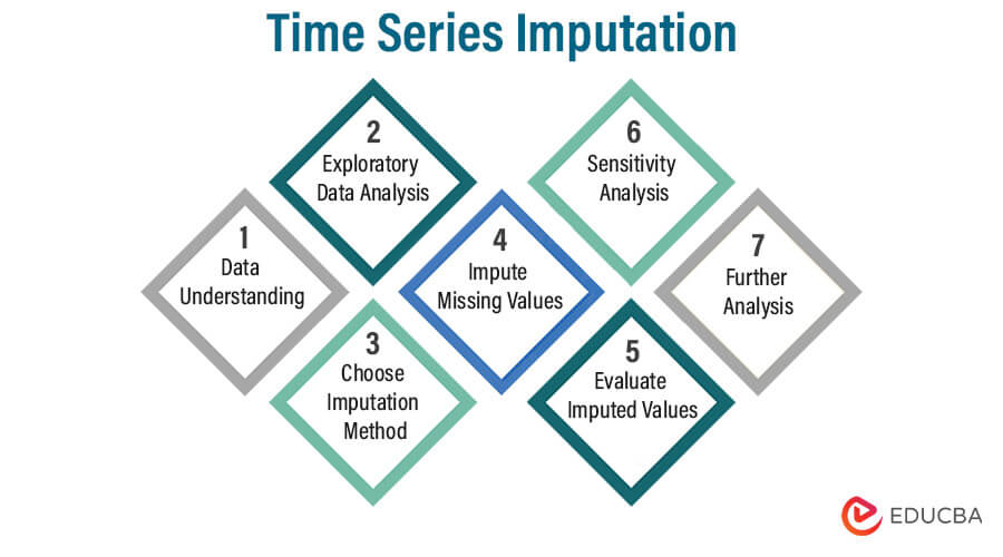
Time Series Imputation is a method used to estimate and fill in missing values within a time series dataset. It focuses on preserving the temporal relationships and patterns present in the data while addressing the gaps caused by missing observations.
Steps:
- Data Understanding: Begin by understanding the time series data, its context, and the reasons for missing values.
- Exploratory Data Analysis: Analyze the time series to identify any patterns, trends, and seasonality that can inform the imputation process.
- Choose Imputation Method: Select an appropriate imputation method based on the nature of the data and the identified patterns.
- Impute Missing Values: Apply the chosen imputation method to estimate the missing values in the time series.
- Evaluate Imputed Values: Assess the quality of the imputed values by comparing them to observed values where available.
- Sensitivity Analysis: Conduct sensitivity analyses to assess the impact of different imputation methods and parameters on the results.
- Further Analysis: Once the missing values are imputed, proceed with the intended time series analysis, which could include forecasting, anomaly detection, or trend analysis.
| Advantages | Disadvantages and Considerations |
| Preserves temporal relationships. | Requires domain knowledge |
| Enables continuity. | Sensitivity to method choice |
| Provides a foundation for forecasting. | Limited by missing data mechanism |
When to Use:
- When you have time series data with missing values that need to be filled to enable subsequent analysis.
- When you want to preserve the temporal relationships and patterns within the data.
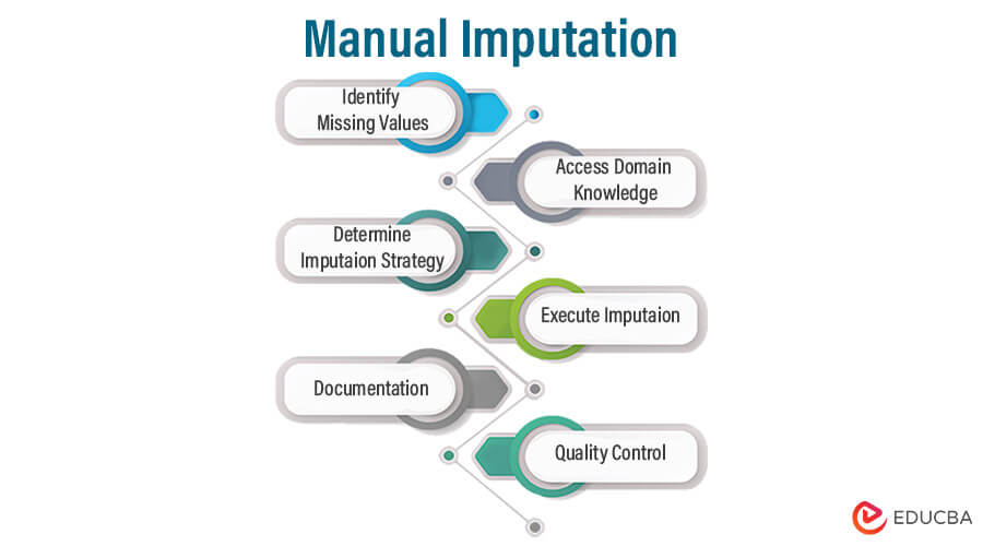
11. Manual Imputation
Manual Imputation is a process in which missing values in a dataset are replaced with estimated values by human experts. It requires domain knowledge, experience, and judgment to make informed decisions about the missing data.
Steps:
- Identify Missing Values: First, identify the variables in your dataset that have missing values that need to be imputed.
- Access Domain Knowledge: Rely on domain knowledge and expertise related to the data and the specific variables with missing values.
- Determine Imputation Strategy: Decide on an appropriate strategy for imputing the missing values.
- Execute Imputation: Based on the chosen strategy, manually enter the estimated values for each missing data point in the dataset.
- Documentation: Keep detailed records of the imputation process, including the rationale behind the imputed values, the expert responsible for the imputation, and any relevant notes or considerations.
- Quality Control: If possible, perform quality control checks or have another expert review the imputed values to ensure consistency and accuracy.
| Advantages | Disadvantages and Considerations |
| Domain expertise. | Subjectivity |
| Flexibility. | Resource-intensive |
| Transparency | Limited to domain expertise |
When to Use:
When you have missing values in a dataset and domain expertise is available to make informed imputation decisions, the dataset contains variables that are context-specific and require deep domain knowledge for accurate imputation.
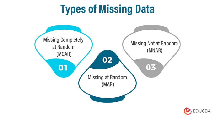
Types of Missing Data
Below are the different types as follows:
1. Missing Completely at Random (MCAR)
In this type, the probability of data being missing is unrelated to both observed and unobserved data. In other words, missingness is purely random and occurs by chance. MCAR implies that the missing data is not systematically related to any variables in the dataset. For example, a sensor failure that results in sporadic missing temperature readings can be considered MCAR.
2. Missing at Random (MAR)
Missing data is considered MAR when the probability of data being missing is related to observed data but not directly to unobserved data. In other words, missingness is dependent on some observed variables. For instance, in a medical study, men might be less likely to report certain health conditions than women, creating missing data related to the gender variable. MAR is a more general and common type of missing data than MCAR.
3. Missing Not at Random (MNAR)
MNAR occurs when the probability of data being missing is related to unobserved data or the missing values themselves. This type of missing data can introduce bias into analyses because the missingness is related to the missing values. An example of MNAR could be patients with severe symptoms avoiding follow-up appointments, resulting in missing data related to the severity of their condition.
Best Practices for Data Imputation
Here are some best practices for data imputation:
1. Exploratory Data Analysis (EDA)
Exploratory Data Analysis (EDA) is a crucial initial step in data analysis, involving the visual and statistical examination of data to uncover patterns, trends, anomalies, and relationships. It helps researchers and analysts understand the data’s structure, identify potential outliers, and inform subsequent data processing, modeling, and hypothesis testing. EDA typically includes summary statistics, data visualization, and data cleaning.
2. Data Visualization
Data Visualization is the graphical representation of data using charts, graphs, and plots. It transforms complex datasets into understandable visuals, making patterns, trends, and insights more accessible. Data visualization aids in data exploration, analysis, and communication by conveying information in a concise and visually appealing manner. It helps users interpret data, detect outliers, and make informed decisions, making it a valuable tool in various fields, including business, science, and research.
3. Cross-Validation
Cross-validation is a statistical technique used to evaluate the performance and generalization of machine learning models. It divides the dataset into training and testing subsets multiple times, ensuring that each data point is used for both training and evaluation. Cross-validation helps assess a model’s robustness, detect overfitting, and estimate its predictive accuracy on unseen data.
4. Sensitivity Analysis
Sensitivity Analysis is a process in which variations in the parameters or assumptions of a model are systematically tested to understand how they impact the model’s results or conclusions. It helps assess the robustness and reliability of the model by identifying which factors have the most significant influence on the outcomes. Sensitivity analysis is crucial in fields like finance, engineering, and environmental science to make informed decisions and account for uncertainty.
Multiple Imputation vs Missing Imputation
| Aspect | Multiple Imputation | Missing Imputation |
| Technique | Generates multiple datasets with imputed values, typically through statistical models. | Imputes missing values once using a single method, such as mean, median, or regression. |
| Handling Uncertainty | Captures uncertainty by providing multiple imputed datasets, allowing for more accurate standard errors and hypothesis testing. | Provides a single imputed dataset without accounting for imputation uncertainty. |
| Avoiding Bias | Reduces bias by considering the variability inherent in imputations and appropriately accounting for it in analyses. | May introduce bias if the imputation method used is not suitable for the data or if the imputed values do not reflect the true distribution. |
| Method Selection | Requires selecting a suitable imputation model, such as regression, Bayesian imputation, or predictive mean matching. | Requires selecting a single imputation method, such as mean, median, or regression, often based on data characteristics. |
| Complexity | More computationally intensive, as it involves running the chosen imputation model multiple times (equal to the number of imputed datasets). | Less computationally intensive, as it involves a single imputation step. |
| Standard Error Estimation | Allows for accurate estimation of standard errors, confidence intervals, and hypothesis testing by considering within- and between-imputation variability. | Standard errors may be underestimated or incorrect due to not accounting for imputation uncertainty. |
| Suitability for Complex | Data is Well-suited for complex data structures, high-dimensional data, and data with complex missing data mechanisms. | Suitable for straightforward data with simple missing data patterns |
| Implementation in Software | Supported by various statistical software packages, such as R, SAS, and Python (e.g., using libraries like “mice” in R). | Widely available in statistical software packages for simple imputation methods. |
Potential Challenges in Data Imputation
Here are some common challenges in data imputation:
- Missing Data Mechanisms: Understanding the nature of missing data is crucial.
- Bias: The imputation method can introduce bias if it systematically underestimates or overestimates missing values.
- Imputation Model Selection: Choosing the right imputation model or method can be challenging, especially when dealing with complex data.
- High-Dimensional Data: In datasets with a large number of features (high dimensionality), imputation becomes more complex.
Future Developments in Data Imputation Techniques
Future developments in data imputation will likely focus on advancing machine learning-based techniques, such as deep learning models, to handle complex datasets with high dimensionality. Additionally, there will be an increased emphasis on addressing missing data mechanisms like Missing Not at Random (MNAR) through innovative modeling approaches.
Conclusion
Data imputation is vital for handling missing data in various fields, ensuring the continuity and reliability of analyses and modeling. While a range of imputation methods exists, choosing the most suitable one requires careful consideration of data characteristics and objectives. With advancements in machine learning and increased awareness of imputation challenges, future developments will likely lead to more robust, transparent, and efficient imputation techniques for addressing missing data effectively.
FAQs
Q1. What are common data imputation methods?
Ans: Common imputation methods include mean imputation, median imputation, k-nearest neighbors imputation, regression imputation, and multiple imputation. The choice depends on data characteristics and research goals.
Q2. What challenges are associated with data imputation?
Ans: Challenges include selecting appropriate imputation methods, handling different types of missing data mechanisms, avoiding bias, addressing high-dimensional data, and ensuring transparency and reproducibility.
Q3. When should data imputation be used?
Ans: Data imputation is used when missing data is present, and preserving data integrity and completeness is essential for analysis or modeling. It is widely used in fields such as healthcare, finance, and social sciences.
Q4 What are the potential pitfalls of data imputation?
Ans: Pitfalls include introducing bias if imputation is not done carefully, misinterpreting imputed values as observed, and not accounting for uncertainty in imputed data. It’s essential to understand the data and choose imputation methods wisely.
Recommended Article
We hope that this EDUCBA information on “Data Imputation” was beneficial to you. You can view EDUCBA’s recommended articles for more information.

