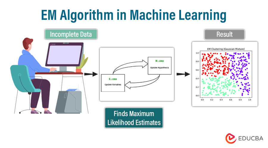
Introduction to EM Algorithm in ML
Welcome to the intriguing world of the EM Algorithm in Machine Learning! If you’re passionate about delving into the depths of data analysis and pattern recognition, you’ve come to the right place. The EM Algorithm, short for Expectation-Maximization Algorithm, stands as a cornerstone in the realm of unsupervised learning, offering a powerful approach to tackle complex problems such as clustering, missing data imputation, and density estimation.
But what exactly is the EM Algorithm, and why is it such a revered tool among data scientists and machine learning enthusiasts? The EM Algorithm is a versatile technique that shines in scenarios where data is incomplete or involves unobservable variables. Its ability to gracefully handle such challenges and extract meaningful insights from the data makes it a valuable asset in the machine learning toolkit.
Throughout this journey, we’ll unravel the inner workings of the EM Algorithm, explore its applications across various domains, and address common questions that arise when venturing into its realm. So, get ready to embark on a captivating exploration of the EM Algorithm in Machine Learning!
Table of Contents
Key takeaways:
- Estimates parameters in a probabilistic model deal with latent variables
- Learn and predict missing data from available data
- Follow the iterative process to compute the expected value of a latent variable
- With each iteration bring the solution closer to convergence
- Terminate when convergence occurs
Concept of EM Algorithm in Machine Learning
The Expectation-Maximization (EM) algorithm stands as a cornerstone in machine learning, adept at handling incomplete or missing data and refining parameter estimates in probabilistic models. Originating in a landmark 1977 paper by Arthur Dempster, Nan Laird, and Donald Rubin, EM has since become indispensable in statistical modeling, particularly in scenarios with latent variables.
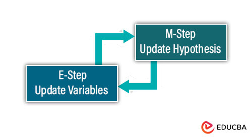
At its essence, EM operates through an iterative approach, alternating between two pivotal phases:
- Expectation Step (E-step): This initial phase estimates the latent or missing variables based on the current model parameters. By computing the expectation of the complete data log-likelihood using the present parameter values, EM advances toward refining its understanding of the underlying data structure.
- Maximization Step (M-step): Following the E-step, EM proceeds to upgrade the model parameters to maximize the anticipated log-likelihood computed in the preceding phase. Typically, this entails optimizing the expected complete data log-likelihood concerning the parameters, pushing the algorithm closer to convergence.
Through iterative repetition of these steps until convergence, where parameter estimates stabilize, EM adeptly navigates the challenges posed by missing or incomplete data, yielding robust parameter estimates. Widely deployed in machine learning, EM finds application in diverse tasks such as clustering (e.g., Gaussian Mixture Models), managing missing data, and training models like Hidden Markov Models.
In real-world machine learning applications, it’s common for certain variables to remain unobserved during the learning process. EM leverages observed variables from instances to infer and predict the unobserved variables, thereby enabling accurate estimation and prediction. This ability to handle latent variables not directly observable stands as one of EM’s defining strengths.
The Expectation-Maximization algorithm’s significance lies in effectively handling missing data, leveraging observed variables to infer latent ones. By amalgamating various unsupervised machine learning algorithms, EM facilitates the determination of local maximum likelihood estimates (MLE) or maximum posterior estimates (MAP) for non-observed variables.
Basics of the EM Algorithm
The Expectation-Maximization algorithm is an iterative statistical technique for handling latent or unobserved variables. This model is used in machine learning or statistics to find the maximum likelihood estimates of variables. This algorithm handles the partially observed variables, and the EM algorithm utilizes the available instance variables to predict the latent variables with the known general form of probability distribution governing these latent variables. The EM algorithm is vital in handling missing data using a simple iterative approach to achieve convergence.
A. Expectation-Maximization Iterative Process
EM algorithm learns patterns from observed data and estimates the value of unobserved data. It operates iteratively in two main steps that are the Expectation step and the Maximization step. The E-step of the algorithm estimates the latent variable based on the observed data, and the M-step of the algorithm updates the parameter from the estimated latent variables.
1. Initialization Step
Initialize the algorithm by providing meaningful values for the model’s parameters and incomplete datasets to start the iterative process. Algorithm convergence is dependent on the initial values. These values can be provided by random guesses, some prior knowledge, or outcomes from other algorithms.
2. Expectation (E) Step
The E-step of the algorithm estimates the expected value of the missing data or latent variable by utilizing the observed data.
- The algorithm computes the posterior probability of each latent variable, considering the observed data and current parameter estimates.
- The posterior probability depicts the likelihood of each latent variable. To calculate the posterior probability, we use Bayes’s theorem.
- With computed posterior probability, the EM algorithm estimates the missing data values.
- The EM algorithm estimates the log-likelihood of the observed data using the current parameter estimates.
- This observed data receives updates with new observations for further processes at the maximization step.
3. Maximization (M) Step
The M-step updates the parameter values using the generated data from the E-step of the algorithm.
- The Maximization step of the algorithm uses the complete data generated from the E-step to update the model’s value.
- The important task of the M-step is to maximize the likelihood by combining the observed data and estimates of latent variables acquired from the E-step
- It updates the parameters of the models by using the complete expected data log-likelihood
- The M-step iteratively refines the model fit to the observed data
- The E-step and M-step undergo iterative repetition until the convergence in values occurs.
B. Mathematical Formulation
1. Likelihood Function
The EM algorithm iterates to maximize the likelihood functions representing the probability of observing data given the sets of parameters in the model.
- We mathematically define the likelihood function as the probability density function of the observed data conditioned on the model parameters, represented by L(θ/X).
- The task of the EM algorithm is to maximize the likelihood function by estimating the parameter value that maximizes the probability of the given data.
- The expectation step of the algorithm computes the likelihood of observed data by providing parameter estimates and latent variables.
- The Maximization step updates the parameter values, maximizing the likelihood function.
2. Incomplete Data
Incomplete data refers to the missing or unobserved variable in a dataset. The EM algorithm carefully handles incomplete data by iteratively estimating the disappeared value by computing the expected data.
- In many scenarios, completing data might be necessary due to measurement error, censoring, or other reasons.
- The EM algorithm task handles incomplete data by estimating missing values based on the current model parameters and observed data.
- In the EM algorithm, the task of the E-step is to compute the expected values of the latent variable from the initial values provided.
- The M-step uses the complete data generated from the E-step and updates the parameters with the estimated missing data value.
- We continue this iterative process until refining the missing values to fit the observed data and achieve convergence with the algorithm.
3. Missing Data and Latent Variables
Missing data refers to the situation where some variables from the dataset remain unobserved or missing. The latent variables are the unobserved variables that are not directly observed but inferred from other observed values. The EM algorithm estimates the value of missing data and latent variables by updating the values of model parameters.
- The algorithm assumes missing data as part of the distribution of observed data and estimates the missing data values through an iterative process.
- The E-step of the algorithm estimates the values for both the observed and latent variables, and the M-step updates the model parameters.
- The algorithm iteratively handles missing data and latent variables to improve overall accuracy and achieve convergence in the algorithm.
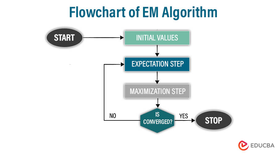
Flowchart of EM Algorithm:
Explanation:
Initialization:
Initialize the algorithm by providing meaningful initial values for model parameters.
Expectation step:
The expectation stage estimates the expected value of a latent variable or missing data by using the current parameters and observed data
Maximization step:
The maximization step uses the expected value generated from the expectation step and updates the model parameter to maximize the likelihood function
Convergence check:
The converged step checks if the change in the parameter is below the predetermined threshold or if the maximum number of iterations has reached
If the convergence criteria have been met, the algorithm terminates or returns to the expectation step and repeats the E-M steps.
Working of EM Algorithm in Machine Learning
Let us understand the mechanism of the Expectation-Maximization algorithm, which combines various unsupervised Machine Learning algorithms to estimate the local maximum likelihood estimates for variables that remain unobserved in the statistical model. In this process, unobserved variables, acting as latent variables, are inferred from the predicted observed variables. The estimated data then updates the parameter value.
It is also known as a latent variable model to find the local maximum likelihood estimates of parameters in an instance with the missing or unobserved data by using the data from the available instance variable.
Step 1 Initialization: The initialization step is crucial in the EM algorithm as it significantly impacts the convergence and outcome. Initialize the algorithm with the set of parameter values. Provide the system with an observed incomplete dataset, assuming data generated from a specific model.
Step 2 Expectation-step: The expectation stage estimates the expected values of latent variables or missing data, leveraging the current parameters and observed data.
- The E-step iteratively refines the parameter estimates during the execution process of the EM algorithm.
- The e-step calculates each latent variable’s responsibilities based on the observed data and current parameter estimates.
- It calculates the posterior probability to represent the likelihood of each latent variable value.
- The E-step of the algorithm iteratively updates the latent variable by utilizing the provided information.
Step 3 Maximization-step: The maximization step uses the complete data generated from the Expectation step to update the parameter value and further update the hypothesis
- The M-step finds the parameter to maximize the log-likelihood of the observed data.
- It updates the parameters of the models by using the complete expected data log-likelihood
- The optimization techniques utilized in M-step depend on the nature of the problem.
- The M-step iteratively refines the model fit to the observed data by maximizing the log-likelihood.
- Both the E-step and M-step go through multiple iterations until values converge.
Step 4 Convergence: After wrapping the E-step and M-step, the last step of the algorithm checks if the values generated are converging or not.
- The Algorithm verifies if the values of the latent variable generated from both above E-M steps are converging or not.
- If the values for the parameters fall below the specified threshold, meeting the criteria for convergence, the outcome will receive a “yes,” and the process will halt or terminate.
- If the algorithm fails to achieve convergence, it will iterate through the E-step and M-step until it reaches convergence and then terminate after producing a stable solution.
Properties of EM Algorithm
The Expectation-Maximization algorithm works on multiple properties as follows:
Sensitive initialization:
Choosing the initial parameter value and the latent variable is sensitive in the E-M algorithm as it can significantly impact the convergence of the solution if initial values are very far from the true values.
- Poor initial values may converge to local optima or slow convergence
- Initial values should be meaningful, particularly for complex models or high-dimensional spaces where likelihood estimates may have multiple local maxima
- To mitigate the initialization sensitivity, employ robust initialization techniques such as K-means clustering, hierarchical clustering, or using any prior knowledge
- Initializing with robust techniques for meaningful values is crucial in the EM algorithm to ensure stable solutions and avoid getting stuck in suboptimal solutions.
Model-based:
The EM algorithm is model-based as it assumes specific probabilistic model data for initializing the parameter and latent variables, making it necessary to have prior knowledge of the data processing model.
- Choosing a model depends on the problem domain and the characteristics of the data.
- The models encapsulate the data distribution and guide the parameter estimation process.
- Any prior knowledge of the model improves parameter estimation accuracy and avoids poor performance.
- Gaussian Mixture models and Hidden Markov models are commonly used in the EM algorithm to avoid biased parameter estimation.
Iterative solution:
The algorithm iterates the Expectations and maximization steps to increase the likelihood function. It iterates both main steps, gradually improving the parameter estimates.
- The iterative nature of the EM algorithm refines the parameter estimates and maximizes the likelihood function.
- The algorithm iterates through both steps alternatively to update parameter estimates until the convergence in value occurs.
- The algorithm’s E-step computes the latent variable’s expected value with the current parameter estimates.
- The M-step of the algorithm updates the parameter based on the generated value from the E-step
- The iterative steps continue until the convergence occurs to improve the model fit to observed data.
Convergence:
Under favorable circumstances, the EM algorithm converges to a stable solution. It determines the local maximum likelihood estimates with a finite number of iterations, and the algorithm repeats the E-step and M-step until convergence occurs.
- The EM algorithm’s last step and critical property is convergence to provide a stable solution.
- The EM algorithm converges to the local maximum likelihood function instead of the global maximum.
- The convergence criteria consist of changes in log-likelihood or values for parameters to fall below a certain threshold.
- It is essential to monitor the stable solution, and techniques like log-likelihood plots, convergence diagnostics, and assessing parameter changes help to determine the final solution.
Applications of EM Algorithm:
1. Gaussian Mixture Model (GMMs):
The EM algorithm is widely used in clustering algorithms to estimate data with similar characteristics and handle uncertainties. It calculates the Gaussian density, weight, shape, and location of each Gaussian components cluster by capturing clustering characteristics.
For example, it is used in target marketing strategies to identify different groups of customers based on their purchasing behavior, such as product preference, amount spent, buying frequency, etc.
2. Hidden Markov Models (HMMs):
The Hidden Markov Model is a probabilistic model mainly used for sequential data analysis where hidden states influence the observed data. EM estimates the parameters of HMMs, which are Emission probabilities and Transition probabilities.
Used for speech recognition, bioinformatics, and finance.
For example, used in speech recognition for identifying phonemes and acoustic features of audio signals, the EM algorithm can transcribe the verbal word into text.
3. Natural Language Processing (NLP):
In natural language processing, practitioners utilize the Expectation-Maximization algorithm for diverse tasks, including text categorization, sentiment analysis, machine translation, topic modeling, and part-of-speech tagging. EM algorithm aids in extracting meaningful insights from text content by analyzing and learning its pattern.
For example, NPL can efficiently identify sentiments in text by reviewing and classifying social media posts into positive, negative, or neutral.
4. Computer Vision:
Computer vision employs the EM algorithm to recognize objects and reconstruct images. It enables us to extract valuable information from the visual data and image content.
For example, the EM algorithm aids in reconstructing a three-dimensional image from a two-dimensional image, and these images can be any medical scans like CT or MRI, which can enhance visualization of any injuries or disease by reconstructing the process.
5. Quantitative genetics:
The EM algorithm allows us to model the genetic information and estimate the gene expression and inheritance pattern parameters. It enables us to understand complex traits and diseases based on genetics.
For example, EM-based algorithms analyze a patient’s medical history to identify genetic markers associated with any health issue. These methods extract valuable information for examining the genetic factors of any disease like diabetes or cancer.
6. Health and Medical Industry:
The EM algorithm has a valuable use in the health care and medical industry for improving patient treatment and care by aiding the detailed information for diagnosis by reconstructing and enhancing the diagnosed image quality.
For example, the EM algorithm helps oncologists in cancer radiation therapy reconstruct a three-dimensional tumor image from a CT scan to target only the affected area and avoid any healthy tissue damage.
7. K-means clustering vs. EM clustering:
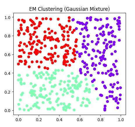
K-means clustering and EM clustering are unsupervised algorithms that group data by iterative process into clusters based on similarities.
Algorithm:
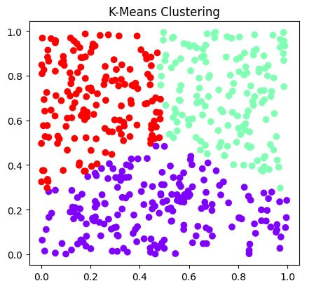
K-Means Clustering: The K-means is an efficient algorithm that simply assigns each data point to the nearest cluster center and updates the centroids based on the mean of assigned points. These cluster algorithms partition data points into K clusters by minimizing the within-cluster sum of the square.
Expectation-maximization clustering: EM clustering can cluster data with complex or mixed distribution. EM clustering, also called GMM, assumes that data originates from a mixture of Gaussian distributions, with each distribution representing a cluster. EM clusters process iteratively to estimate the parameters of this Gaussian distribution to maximize the likelihood.
Sensitive initialization:
K-means clustering: K-means clustering is sensitive to the initialization of cluster centroids, as different initializations may lead to different cluster assignments.
EM clustering: EM is sensitive to the initialization for the means and covariance of Gaussian distribution. The probabilistic nature of EM can handle the initialization issue.
Computational Complexity:
K-Means Clustering: The computational complexity of K-means is O (I*K*N*D). Here,
I is the iteration number, K is the number of clusters, N is the number of data points, and D is the dimensionality of Data.
EM clustering: The computational complexity of EM is O (MN), which depends on the number of iterations and convergence criteria. The iterative nature and probabilistic modeling provide higher complexity for EM clustering.
Convergence:
K-means clustering: K-means clustering converges to the local minimum of the within-cluster sum of squares. Convergence occurs when cluster centroids remain unchanged. K-Means generates clusters with uniform variance and shape.
EM clustering: EM clustering converges to the local maximum of the likelihood function. Convergence occurs when the log-likelihood change falls below a specific threshold. EM demonstrates greater flexibility in dealing with clusters of different shapes and sizes.
8. Density Estimation:
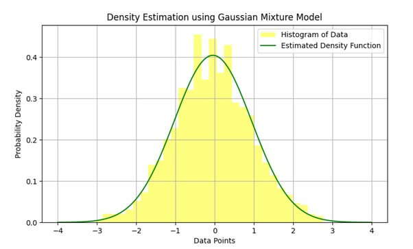
Density estimation is the process of estimating the Probability distribution function of a random variable from the available data, and this estimation process handles the latent variable. In density estimation, the EM algorithm iteratively estimates the parameter of a probabilistic model that best fits the observed data.
For example, density estimation can be used in anomaly detection systems to detect any unusual pattern in data that can indicate any fraudulent activity or system failure.
The graph below represents the data histogram and the estimated Probability distribution function obtained from GMM using the EM algorithm:
Gaussian Mixture Model (GMM)
The Gaussian mixture model is a probabilistic model, and it is a mixture model consisting of the distribution of data as a mixture of several Gaussian distributions. This mixture model consists of an unspecified probability distribution function. The Gaussian components represent clusters within the data, and a learning algorithm estimates the parameter (mean, covariance, and weight) of a probability distribution to best fit the density of the provided dataset. A Maximum Likelihood Estimation (MLE) is the most commonly used technique to estimate the parameters of the Gaussian Mixture Model.
Implementing Gaussian Mixture Models in Python
Code:
import numpy as np
import matplotlib.pyplot as plt
from sklearn.datasets import make_blobs
from sklearn.mixture import GaussianMixture

X, _ = make_blobs(n_samples=200, centers=4, cluster_std=0.50, random_state=0)
gaussian = GaussianMixture(n_components=4, random_state=42)
gaussian.fit(X)
labels = gaussian.predict(X)

plt.scatter(X[:, 0], X[:, 1], c=labels, cmap='rainbow')
plt.colorbar(label='Cluster')
plt.title('Gaussian Mixture Model (GMM)')
plt.show()
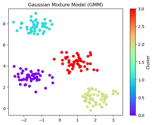
Output:
Explanation:
- Import the essential library to generate datasets with cluster and a fitting class for the Gaussian Mixture Model.
- The ‘make_blobs’ function generates synthetic data points with a cluster by setting parameters to create different datasets.
- Initialize GMM with specific number clusters and use class for fitting GMM to data.
- Use the ‘predict’ method to assign labels for each data point.
- Use the ‘scatter’ function to plot data points and the color mapping parameter to color the data point based on its assigned cluster label.
Advantages and Disadvantages
Advantages:
1. Flexibility: The EM algorithm is a diverse framework that applies to various statistical and probabilistic models. This algorithm has great use in clustering, density estimation, parameter estimation, and even handling missing or latent variables. EM algorithm employs complex data distribution and relationship by iteratively estimating the local maximum likelihood parameters.
2. Latent Variable: The main benefit of the EM algorithm is its capability to handle missing data or latent variables seamlessly. EM algorithm estimates the unobserved or missing data from the observed data. It processes iteratively to update the parameter value, leading to accurate allocation. This ability of the EM algorithm makes it useful for handling scenarios with unobserved data.
3. Iterative Convergence: The EM algorithm processes iteratively to refine the parameter estimates until convergence. Each iteration of the EM algorithm increases the likelihood of the observed data, making it the best fit for the model. The algorithm’s iterative process ensures improvement after each iteration, leading to accurate parameter estimates.
4. Probabilistic Framework: The EM algorithm allows data modeling using a probabilistic framework such as Gaussian distribution. This algorithm estimates the probability distribution of parameters based on the observed data. EM algorithm generates a posterior probability of a cluster representing the likelihood of each data point belonging to different clusters. The probabilistic nature of the EM algorithm ensures efficient decision-making and analysis of uncertainties in data modeling.
Disadvantages:
1. Sensitive initialization: The performance of the EM algorithm depends on the initialization of parameter values. The algorithm’s convergence is highly sensitive to the initial values as different initializations may lead to other local optima impacting the final solution. The initialization sensitivity of the algorithm is due to the iterative process of the E-M step, which updates the values of parameters on the estimation from the observed data provided at initialization.
2. Computational complexity: The EM algorithm processes iteratively through the E-step and M-step, which can be computationally intensive. Complex models or large datasets require enormous numbers of iterations to achieve convergence. The iterative nature of the EM algorithm increases the computational complexity as it needs a significant amount of computational time and resources.
3. Convergence Issues: Obtaining convergence in the EM algorithm is sometimes challenging as the criteria of convergence based on the changes in likelihood or parameter estimates may sometimes lead to convergence failure. An ill-conditioned model or poor representation of data distribution may result in slow convergence or variation in parameter estimates. Proper initialization, convergence monitoring, and criteria are required to ensure convergence.
4. Sensitive to Outliers: The EM algorithm can be easily affected by outliers or noise in data, particularly in Gaussian distribution models. Outliers may immoderately affect parameter estimates, resulting in biased outcomes and lowered model performance. Steady method and proper techniques are required to reduce the effect of outliers on parameter estimation.
Benefits and Limitations
Benefits
Easy Implementation
The EM algorithm follows simple steps to achieve a stable solution. Both the main steps of the EM algorithm work in a straightforward manner while being implemented in different machine-learning problems. The expectation step computes the expected value of data from the observed data, and the maximization step updates the parameter value from the generated data. The simple application of the EM algorithm makes it easily accessible to various statistical models and machine-learning tasks.
Enhance Likelihood
The EM algorithm maximizes the likelihood function of observed data with each iterative step. It guarantees the enhancement in the likelihood after each iteration, leading to the converged solution. The algorithm ensures the solution converges to the local maximum likelihood of functions by increasing the parameter estimates with each iteration.
Closed-form Solution
The EM algorithm can lead to a closed-form solution for parameter updates, resulting in fast convergence. Analytical solutions eliminate the necessity for iterative numerical optimization, reducing computational time and complexity.
Handle incomplete data.
The EM algorithm provides a robust solution, even partial information. It handles the dataset with incomplete information by iteratively estimating the missing data and refining the parameters.
Limitation
Slow convergence:
The EM algorithm converges slowly, particularly in high-dimensional and complex parameter instances. Converging to a local maximum likelihood of function algorithm requires many iterations, leading to slow convergence compared to other optimal algorithms. Slow convergence becomes challenging for applications with critical time and computational efficiency. It increases the computational time for estimating parameters, making the algorithm less efficient and sensitive in real time. Some techniques like efficient initialization, optimizing convergence criteria, or parallelizing computation can avoid these limitations and boost convergence.
Local Optima:
The EM algorithm, mainly with complex parameters, converges to the local maximum rather than the global maximum, resulting in a suboptimal solution. Poor initialization and multiple peaks in the likelihood function may result in suboptimal solutions. This requires running the algorithm multiple times with various initializations to mitigate the convergence issue. Convergence to local optima impacts the quality of the solution and limits the algorithm to suboptimal solutions. Strategies like performing multiple runs with different initialization or employing advanced optimization algorithms are proposed to overcome these limitations to achieve likelihood functions.
Consideration of Forward and Backward Probabilities:
The EM algorithm considers both the forward and backward probabilities, unlike the traditional method, which only considers forward probabilities. The twofold probabilities for estimating parameters are considered in an application such as hidden Markov models. This consideration of the EM algorithm may require more computational time and complexity with large datasets. The forward and backward probabilities require dynamic programming techniques, which can be computationally intensive and slow the algorithm’s convergence process. Optimizing the implementation of a forward-backward algorithm or using more efficient methods can help improve the performance of the EM algorithm in HMM models.
Require sufficient data:
The EM algorithm estimated the data based on the provided data, and to calculate the parameters accurately, the algorithm requires a sufficient amount of data. The algorithm needs to work on delivering the optimal solution in scenarios with small datasets and less observation for latent variables. Insufficient data can lead to overfitting or underfitting of the model, and it’s crucial to balance the model complexity with the available amount of data to achieve convergence.
Comparisons with Other Algorithms
| Features | EM algorithm | K-Means | Hierarchical clustering | GMM | HMM |
| Cluster nature | Soft clustering | Hard Clustering | Hierarchical clustering | Soft clustering | Temporary clustering |
| Numbers of clusters | Depend on implementation | Predefined (K) | Determine while clustering
|
predefined | Depending on the structure of the model |
| Latent variable | Yes | No | No | Yes | Yes |
| Computational complexity | Moderate | Fast | High | Moderate | High |
| Data sensitivity | Handle data with E-step | Not robust | Sensitive | Handle with EM-based substitution | Sensitive |
| Computational cost | Depend on implementation | Efficient | Relatively high | More higher than K-Means | Depending on the model complexity |
| Interpretability | Probability distribution of data | Centroids | Hierarchical structure | Probability distribution of clusters | Transition and emission |
| Applications | Diverse use depends on the implementation | Image segmentation and data exploration | Data analysis | Density estimation, anomaly detection | Sequence analysis and speech recognition |
| Time Complexities | O(k⋅n⋅m⋅d) | O(k⋅n⋅m⋅d) | O(n^2 . log n) to O(n^3) | O(k⋅n⋅m⋅d⋅iterations) | O(T.N^2) |
Case Studies
Case Study: Image segmentation using Gaussian Mixture models
Image segmentation:
Image segmentation is a fundamental part of computer vision that partitions images into multiple segments for easy and simplified representation and analysis. Gaussian Mixture models provide a powerful approach for segmenting images by modeling pixel intensities in different image segments.
Problem statement:
Use Gaussian Mixture models to segment an image into multiple regions based on pixel intensities to identify different regions or objects in an image.
Algorithm overview:
The Gaussian Mixture model (GMM) is a probabilistic model for modeling the pixel intensities in different regions of images, these probabilistic frameworks represent the probability distribution of provided datasets as a mixture of several Gaussian distributions. GMM allows image segmentation which is essential in various sectors like object recognition, medical imaging, and scene understanding.
Methodology:
- Data preparation and pre-processing:
Load an image to perform the segmentation process. Pre-process images by providing uniform size, filtering noisy images, and converting to grayscale if necessary.
- Feature Extraction:
Extract features from an image by representing each pixel in the image as a feature vector, such as color information, intensity values, etc.
- Model training:
Train the GMM algorithm on a subset of the dataset using the EM algorithm to estimate the model parameter. Apply GMM with EM algorithm to the extracted features from images. Initialize the GMM with the desired number of Gaussian components by some prior knowledge or a model selection technique.
- Segmentation:
Assign each pixel in the image to each Gaussian component, and segment these images into different regions based on their color distribution. Pixels are assigned to the components with the highest probability, maximizing its likelihood by using trained GMM.
- Post-processing:
To post-process segmentation apply Morphological operations to refine the segmentation mask and remove small artifacts to ensure spatial coherence in the segmented regions.
- Visualization:
Assign each pixel with a unique color to the corresponding segment label to visualize the segmented region and display the segmented image along with the original image for segmentation comparison.
Example Scenario:
Let’s take an example of performing image segmentation on a landscape image:
Code:
import numpy as np

import cv2

from sklearn.mixture import GaussianMixture

image = cv2.imread('landscape_image.jpg')

pixels = image.reshape(-1, 3)

num_clusters = 4

gmm = GaussianMixture(n_components=num_clusters, random_state=40)

gmm.fit(pixels)

labels = gmm.predict(pixels)

segmented_image = labels.reshape(image.shape[:2])

cv2.imshow('Original Landscape Image', image)

cv2.imshow('Segmented Landscape Image', (segmented_image * (255 // num_clusters)).astype(np.uint8))

cv2.waitKey(0)

cv2.destroyAllWindows()
Output:
After Segmentation:
Explanation:
- Import Libraries: Import necessary libraries for numerical computation, computer vision, and implementation of the GMM
- Data preparation: Load the landscape image for performing segmentation
- Feature Extraction: Reshape the image into a two-dimensional array of pixels with rows representing pixels and columns representing RGB channel
- Model Training: Define the number of clusters to segment the image into four segments—Initialize GMM with the components (num_cluster). Fit the GMM model to the pixel data.
- Segmentation: Assign each pixel image to the GMM components based on the likelihood of its RGB values.
- Visualization: Display the original and the segmented image. Reshape the original image before reshaping.
Conclusion:
The EM algorithm is a simple approach in machine learning to estimate the latent variable or missing data from available data in any probabilistic model. The iterative nature, soft clustering capabilities, and application in Gaussian Mixture Models make it integral in various domains. Despite challenges like slow convergence and local optima, EM remains an adaptable and essential algorithm.
Frequently Asked Questions (FAQs)
Q1). What are outliers, and how can they be handled?
Answer: In the given set of data, some unusual data points differ from the set, such that they have incredibly high and low values. Hence, to handle such data, techniques differ from usual. Instead, EM makes guesses and defines a model based on probability. Robust mixture models are also utilized when outliers exhibit extreme values, as these outliers can impact the performance of the EM algorithm. These models are less sensitive as compared to traditional models. These steps involve pre-processing detection of outliers; if detected outliers are very extreme, they can also be eliminated. Some of the robust mixture models are the Robust Gaussian Mixture model (GMM), Mixture of Factory Analyzer (MFA), Mixture of Experts (MoE), etc.
Q2). What are specialized versions of the Expectation Maximization algorithm to handle time series data?
Answer: There are many extended versions of the Expectation Maximization algorithm to handle time series data as outlined below:
1) Hidden Markov Models (HMM) – HMM is one of the most widely used models to handle time series data. Hidden Markov Models (HMMs) fall into the category of probability-based models, making the EM algorithm a common choice for predicting parameters in HMMs. It serves to compute the transitioning probabilities between hidden states as they change.
2) Kalman Filters and Kalman smoothers – These repetitive algorithms predict linear dynamic states from a series of disturbed noisy datasets.
Some other models are the Aautoregressivemodel and the Sstatespace model.
Q3). In Machine learning, what techniques exist to accelerate convergence in the EM algorithm?
Answer: Many techniques accelerate convergence in the EM algorithm.
1) Initialisation – Properly defining the parameters using k-means clustering or multiple restarts accelerates convergence.
2) Accelerated EM – The EM algorithm is modified using information from previous iterations, which helps in accelerating convergence.
3) Parallelization – Managing computations and calculations across several processors using parallel versions of EM helps convergence acceleration.
Other techniques are step size adaption, Regularisation, Variational EM, Mini batch EM, etc.
Recommended Articles
We hope that this EDUCBA information on the “EM Algorithm in Machine Learning” was beneficial to you. You can view EDUCBA’s recommended articles for more information.
