Introduction
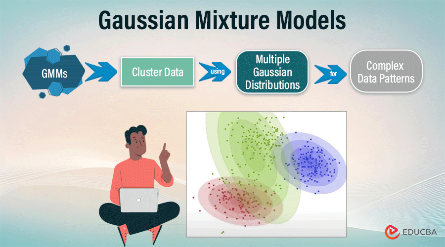
The Gaussian Mixture Model (GMM) is a versatile statistical model utilized across various domains, offering a flexible approach to modeling complex data distributions. It operates on the premise that we can often represent data as a mixture of several Gaussian distributions, each contributing differently to the overall distribution. GMMs find applications in tasks such as clustering, density estimation, and anomaly detection, owing to their capability to capture intricate data structures. Using the Expectation-Maximization (EM) algorithm, GMMs estimate parameters such as means, covariances, and mixing coefficients from the observed data. This introductory overview sets the stage for delving into the mathematical formulation, workings, applications, and advanced topics surrounding Gaussian Mixture Models.
Table of Contents
Intuition Behind Gaussian Mixture Models
Basic Idea
The concept underlying Gaussian Mixture Models (GMMs) centers on their capacity to depict intricate data distributions by amalgamating elementary Gaussian distributions. Picture a scenario where data points showcase patterns that defy simple characterization by a single Gaussian distribution. GMMs tackle this challenge by positing that the data originates from a blend of numerous Gaussian distributions, each denoting a separate underlying cluster or element. By amalgamating these Gaussian components, each with distinct means and variances, GMMs effectively encapsulate the underlying data structure, accommodating scenarios where data exhibits multimodal characteristics or complex patterns.
Example
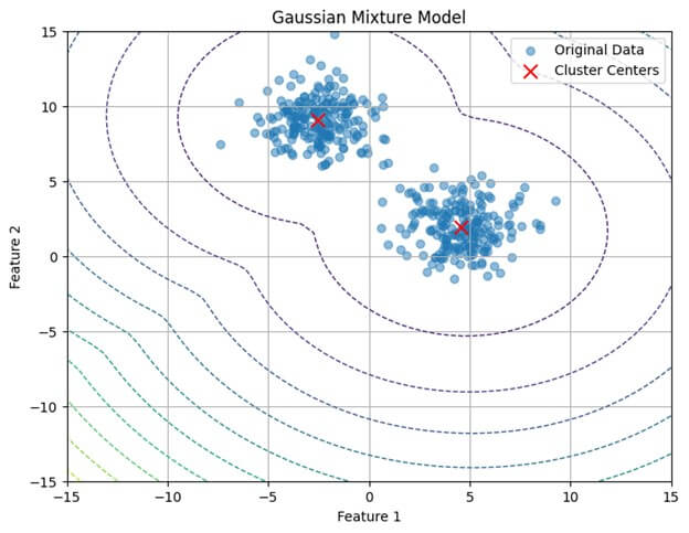
Imagine a dataset with two distinct clusters, each resembling Gaussian distributions but overlapping significantly. A single Gaussian model fails to represent this complexity accurately. Enter the Gaussian Mixture Model (GMM). By conceptualizing the dataset as a blend of two Gaussian distributions, GMM effectively captures the intricate relationships within the data. Through Scikit-learn, we fit a GMM with two components to the dataset. The resulting visualization demonstrates how GMM discerns the boundaries between overlapping clusters, providing a nuanced understanding of the underlying data structure. This example illustrates the power of GMM in modeling complex data distributions and its application in various analytical tasks.
Types of Mixture Models
Mixture models represent a diverse set of statistical models that posit data as originating from a blend of multiple underlying probability distributions. While Gaussian Mixture Models (GMMs) are prominent in this category, researchers customize various mixture models to specific scenarios and data attributes.
- Gaussian Mixture Models (GMMs): GMMs posit that data distributions are combinations of Gaussian distributions. Renowned for their simplicity and effectiveness, they adeptly capture various data distributions.
- Dirichlet Process Mixture Models (DPMMs): DPMMs extend the concept of mixture models by accommodating infinite components. They excel in situations where the count or variability of clusters/components is uncertain.
- Finite Mixture Models: These models generalize GMMs but impose a fixed number of components. They are advantageous when the count of underlying clusters is either known or estimable.
- Hierarchical Mixture Models: These models introduce a hierarchical organization among components, facilitating the modeling of intricate relationships between clusters across different abstraction levels.
- Bayesian Mixture Models: Bayesian mixture models introduce prior distributions over mixture component parameters, enabling systematic uncertainty quantification and regularization.
- Nonparametric Mixture Models: Relaxing the constraint of a fixed component count, nonparametric mixture models permit the number of components to expand with data size. This adaptability makes them suitable for modeling complex data with varying cluster sizes and shapes.
Mathematical formulation of Gaussian Mixture Models
Gaussian Mixture Models (GMMs) are probabilistic models that represent intricate data distributions by blending numerous Gaussian distributions. The mathematical framework of GMMs encapsulates the probability density function (PDF) and the parameters that govern the model.
Probability Density Function(PDF):
In a GMM, expression of the PDF as a weighted sum of Gaussian distributions:
Where:
- Of the data point is the probability density function.
- Is the total number of Gaussian components in the mixture.
- Signifies the weight or the mixing coefficient associated with the Gaussian component.
- Denotes the Gaussian distribution with mean and covariance matrix.
Parameters:
The parameters of a GMM include the means (), covariances (), and mixing coefficients () of the individual Gaussian components. Estimate these parameters from the given data using the Expectation-Maximization (EM) algorithm.
How Gaussian Mixture Models Work
Gaussian Mixture Models (GMMs) represent complex data distributions by combining multiple Gaussian distributions. To comprehend their inner workings, it’s essential to delve into the Expectation-Maximization (EM) algorithm and convergence criteria, which are fundamental to their functionality.
Expectation-Maximization (EM) Algorithm
The EM algorithm iteratively optimizes the GMM’s parameters by alternating between the Expectation (E) step and the Maximization (M) step.
E-step:
In the E-step, the algorithm computes the expected values of the latent variables, which are the probabilities of each data point belonging to each component of the mixture. Mathematically, the expression is:
Where:
- Represents the probability of data points belonging to a component of the mixture.
- Denotes the mixing coefficient of the component.
- Is the probability density function of the Gaussian distribution with mean and covariance.
M-step:
The algorithm updates the following parameters of the mixture components using the expected values computed in the E-step. M-step calculates the updates using maximum likelihood estimation.
Convergence Criteria
Typically, we determine convergence in the EM algorithm by monitoring the change in the log-likelihood function between iterations. Consider the algorithm to have converged when this change falls below a specified threshold, indicating that further iterations are unlikely to improve the model fit significantly. Expression of the Convergence criterion is:
Where:
- Represents the log-likelihood of the data under the model parameters at iteration.
- is a predefined threshold.
Applications of Gaussian Mixture Models
Gaussian Mixture Models (GMMs) have extensive applications across various fields due to their adaptability in handling complex data distributions. Recognizing the broad spectrum of these applications allows us to grasp the practical relevance of GMMs in real-world contexts.
- Clustering: GMMs are widely employed in clustering tasks to group data points based on similarity. By representing each cluster as a Gaussian distribution, GMMs effectively capture intricate cluster shapes, making them suitable for diverse datasets.
- Density Estimation: GMMs are potent tools for estimating the probability density function of datasets. Their flexible framework accommodates multimodal distributions, facilitating precise estimation of underlying data distributions. This application aids in anomaly detection and outlier analysis.
- Anomaly Detection: GMMs excel in identifying anomalies by modeling the typical behavior of a system and detecting data points significantly diverging from this modeled distribution. Such anomalies exhibit low probability under the GMM, indicating unusual behavior or outliers.
- Natural Language Processing (NLP): In NLP, GMMs play vital roles in tasks like topic modeling and document clustering. By representing documents as topic distributions, GMMs unveil latent structures in extensive text corpora, offering insights into document similarity and topic composition.
- Image Segmentation: GMMs are pivotal in image processing tasks, particularly in image segmentation endeavors to delineate distinct regions or objects. By modeling pixel intensities as Gaussian distributions within each region, GMMs accurately segment images based on intensity resemblances.
Practical Application of GMMs
Gaussian Mixture Models (GMMs) offer practical utility across numerous domains, facilitated by their ability to model complex data distributions. Leveraging the Scikit-learn library in Python, GMMs can efficiently apply for data preprocessing, visualization, and modeling tasks.
Using Scikit-learn
- Scikit-learn, a Python library, provides a robust implementation of Gaussian Mixture Models (GMMs).
- It offers an intuitive interface for fitting GMMs to data, making predictions, and conducting various tasks such as clustering, density estimation, and anomaly detection.
- The GMM module in Scikit-learn allows users to specify parameters such as the number of components, covariance type, and initialization method, providing flexibility to tailor the model as per requirements.
- With its well-documented API and extensive documentation, Scikit-learn simplifies implementing GMMs in real-world applications.
Code:
import numpy as np
import matplotlib.pyplot as plt
from sklearn.datasets import make_blobs
from sklearn.mixture import GaussianMixture

# Generate synthetic data
X, _ = make_blobs(n_samples=400, centers=4, cluster_std=1.0, random_state=42)

# Fit Gaussian Mixture Model
gmm = GaussianMixture(n_components=4, random_state=42)
gmm.fit(X)
Data Preprocessing and Visualization
Before applying Gaussian Mixture Models (GMMs) to data, preprocessing is essential to ensure the data is appropriately formatted and scaled for modeling. Common preprocessing steps include:
- Scaling: Standardizing or normalizing the data to ensure that all features have a similar scale, preventing features with larger magnitudes from dominating the model’s learning process.
- Dimensionality Reduction: Methods such as PCA or t-distributed Stochastic Neighbor Embedding (t-SNE) can decrease the data’s dimensionality while retaining its fundamental features, simplifying its representation for modeling purposes.
- Handling Missing Values: Dealing with missing or null values in the dataset through imputation or removal ensures that the data is complete and suitable for analysis.
Visualization is pivotal in comprehending data characteristics and pinpointing potential clusters before implementing GMMs. Techniques like scatter plots, histograms, and heatmaps offer valuable insights into data distribution, unveiling patterns, correlations, and prospective clusters. Scatter plots elucidate the relationship between two features or dimensions, while histograms depict the distribution of a single feature. Heatmaps prove beneficial in visualizing pairwise relationships or correlations among features, facilitating feature selection or dimensionality reduction.
Code:
# Visualize the data and GMM clusters
plt.figure(figsize=(8, 6))

# Plot original data points
plt.scatter(X[:, 0], X[:, 1], alpha=0.5, label='Original Data')

# Plot decision boundary
x = np.linspace(-10, 10)
y = np.linspace(-10, 10)
X_grid, Y_grid = np.meshgrid(x, y)
Z = -gmm.score_samples(np.array([X_grid.ravel(), Y_grid.ravel()]).T)
Z = Z.reshape(X_grid.shape)
plt.contour(X_grid, Y_grid, Z, levels=10, linewidths=1, linestyles='dashed')

# Plot cluster centers
plt.scatter(gmm.means_[:, 0], gmm.means_[:, 1], marker='x', color='red', s=100, label='Cluster Centers')

plt.title('Gaussian Mixture Model')
plt.xlabel('Feature 1')
plt.ylabel('Feature 2')
plt.legend()
plt.grid(True)
plt.show()
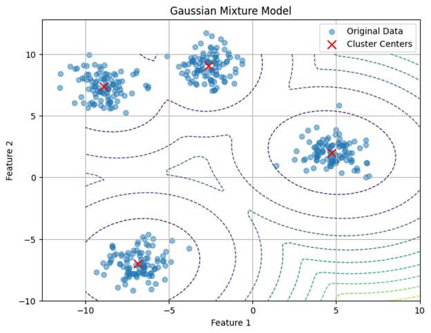
Output:
Code Example for Using GMM in Python
Code
import numpy as np
import matplotlib.pyplot as plt
from sklearn.datasets import make_moons
from sklearn.preprocessing import StandardScaler
from sklearn.mixture import GaussianMixture
from matplotlib.patches import Ellipse

# Generate synthetic data with two moons
X, _ = make_moons(n_samples=400, noise=0.1, random_state=42)

# Preprocess the data (standardization)
scaler = StandardScaler()
X_scaled = scaler.fit_transform(X)

# Fit Gaussian Mixture Model
gmm = GaussianMixture(n_components=2, covariance_type='full', random_state=42)
gmm.fit(X_scaled)

# Predict cluster labels
labels = gmm.predict(X_scaled)

# Visualize the data and GMM clusters
plt.figure(figsize=(8, 6))

# Plot original data points
scatter = plt.scatter(X_scaled[:, 0], X_scaled[:, 1], c=labels, cmap='viridis', alpha=0.5, label='Clustered Data')

# Plot cluster centers
plt.scatter(gmm.means_[:, 0], gmm.means_[:, 1], marker='x', color='red', s=100, label='Cluster Centers')

# Plot ellipses for each cluster
for i in range(gmm.n_components):
    covariances = gmm.covariances_[i][:2, :2]
    mean = gmm.means_[i][:2]
    eigenvalues, eigenvectors = np.linalg.eigh(covariances)
    angle = np.degrees(np.arctan2(*eigenvectors[:, 1]))
    width, height = 2 * np.sqrt(2) * np.sqrt(eigenvalues)
    color = 'yellow' if i == 0 else 'purple'  # Different color for each cluster
    ellipse = Ellipse(xy=mean, width=width, height=height, angle=angle, color=color, alpha=0.3)
    plt.gca().add_patch(ellipse)

# Custom legend for clustered data
legend1 = plt.legend(*scatter.legend_elements(), title="Clusters")

# Custom legend for cluster centers
legend2 = plt.legend(["Cluster Centers"], loc="upper right")

plt.gca().add_artist(legend1)  # Add legend1 back to the plot
plt.title('Gaussian Mixture Model for Clustering')
plt.xlabel('Feature 1 (Standardized)')
plt.ylabel('Feature 2 (Standardized)')
plt.grid(True)
plt.show()
In this example:
- Generate synthetic data with two moons using the make_moons
- Preprocess the data by standardizing it using StandardScaler.
- Train a GMM with two components using the GaussianMixture class on the preprocessed data.
- Predict cluster labels using the trained GMM.
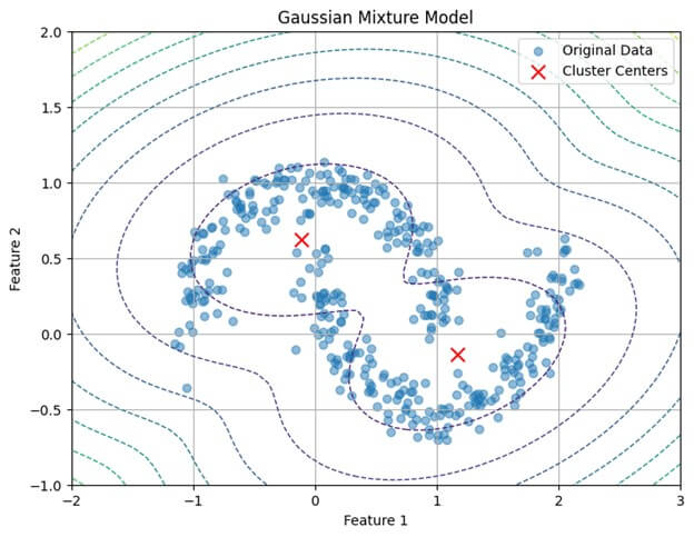
- Visualize the data and GMM clusters using scatter plots, with cluster labels assigned different colors and cluster centers marked in red.
Output:
Choosing the Number of Components
In Gaussian Mixture Models (GMMs), choosing the right number of components is vital for optimal model performance. This selection entails accurately balancing model complexity and capacity to represent the underlying data distribution.
Model Selection Criteria
- Various criteria, including the Akaike Information Criterion (AIC), the Bayesian Information Criterion (BIC), and the likelihood ratio test, can guide the selection of the optimal number of components.
- The AIC and BIC penalize model complexity for preventing overfitting, with lower values indicating better model fit.
- Likelihood ratio tests involve comparing the likelihood of the data across various models, helping identify the most parsimonious model.
Balancing Complexity and Fit
- Increasing the number of components in a GMM can lead to a better fit for the training data, potentially capturing more intricate data distributions.
- However, excessively increasing the number of components can result in overfitting, where the model learns noise in the data rather than meaningful patterns.
- Balancing model complexity and fit is essential by considering the trade-off between model performance and interpretability.
- Employ techniques such as cross-validation or grid search to evaluate the performance of GMMs with different numbers of components and select the model that achieves the best balance between complexity and fit.
Advanced Topics in GMMs
Bayesian Gaussian Mixture Models
- Incorporating prior distributions over model parameters, Bayesian GMMs enable principled uncertainty quantification and regularization.
- Bayesian GMMs facilitate robust parameter estimation and model selection by inferring posterior distributions over parameters.
- Methods commonly employed for posterior inference in Bayesian GMMs include Markov Chain Monte Carlo (MCMC) techniques or variational inference.
Variational Inference for GMMs
- Variational inference presents an alternative to Bayesian inference for GMMs. It approximates the posterior distribution with a simpler, tractable distribution.
- It optimizes parameters to minimize the Kullback-Leibler divergence, offering a scalable and efficient approach for estimating posterior distributions, especially in large datasets.
Handling High-dimensional Data and Scalability Issues
- GMMs encounter challenges when applied to high-dimensional data due to the curse of dimensionality.
- Techniques like dimensionality reduction (e.g., PCA) or feature selection can alleviate these challenges by reducing the number of dimensions.
- Additionally, scalable GMM implementations, such as mini-batch algorithms or distributed computing frameworks, enhance efficiency and scalability for analyzing large datasets.
Conclusion
Gaussian Mixture Models (GMMs) offer a powerful framework for modeling complex data distributions and performing various tasks such as clustering, density estimation, and anomaly detection. Despite their versatility, GMMs have limitations, such as the assumption of Gaussian distribution and sensitivity to initialization. However, by understanding these challenges and employing appropriate techniques for model selection and data preprocessing, practitioners can effectively leverage GMMs for insightful analysis and pattern recognition. With their ability to capture intricate data structures and provide probabilistic interpretations, GMMs remain valuable tools for data scientists and machine learning practitioners.
Frequently Asked Questions (FAQs)
Q1. Are GMMs suitable for high-dimensional data?
Answer: When applied to high-dimensional data, Gaussian Mixture Models (GMMs) may face challenges due to the curse of dimensionality. Methods like dimensionality reduction or feature selection can alleviate these challenges and bolster model performance.
Q2. Can GMMs be used for outlier detection?
Answer: GMMs can serve for outlier detection by pinpointing data points with minimal probability under the fitted mixture model. Outliers typically exhibit low likelihoods within the GMM, signifying their deviation from the modeled data distribution.
Q3. Are there alternatives to GMMs for modeling complex data distributions?
Answer: Various alternatives to GMMs are available, encompassing non-parametric techniques like kernel density estimation, hierarchical clustering algorithms such as agglomerative clustering, and deep learning models like variational autoencoders (VAEs) or generative adversarial networks (GANs). The selection of a method hinges on the data’s unique traits and the analysis’s goals.
Recommended Articles
We hope that this EDUCBA information on “Gaussian Mixture Models” was beneficial to you. You can view EDUCBA’s recommended articles for more information,


