Updated August 10, 2023
ADDRESS in Excel
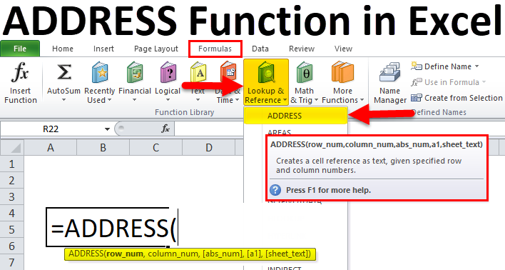
Address Function is a pre-built integrated Excel function categorized under Lookup and Reference functions. Address Function in Excel is used to find out the address of a cell in a worksheet. ADDRESS Function in Excel returns or displays the address of a cell based on a given row and column number.
ADDRESS Formula in Excel
Below is the ADDRESS Formula in Excel :
OR
=ADDRESS (row, column, [ref_type], [ref_style], [sheet_name] )
The ADDRESS Function in Excel has the below-mentioned arguments:
- Row or row_num: (Compulsory or required parameter) It is a row number of the cell address.
- Column or Column_num: (Compulsory or required parameter) It is a column number of the cell address.
- [abs_num] or ref_type: (optional argument) It is a numeric value specified to obtain the reference type below.
Different Types of References
| Value | Explanation |
| 1 or Default | Absolute referencing, e.g., $A$1 |
| 2 | Relative column & absolute row, e.g. A$1 |
| 3 | Absolute column & relative row e.g. $A1 |
| 4 | Relative referencing, e.g., A1 |
- [ref_style] or [a1] : (optional argument) It is a logical value indicating whether to use standard (A1 style) cell reference format or R1C1 style cell reference format. This argument allows you to select the below-mentioned ref_style.
If this parameter or argument is omitted or not entered, it will consider the default value 1 or TRUE (A1 style).
In the A1 reference style, the column name is mentioned as an alphabet, and the row name as a number, Whereas in the R1C1 reference style, both row and column are mentioned in numbers.
- [sheet_text]) or [sheet_name]: (optional argument) It is the name of the worksheet to return. Or the worksheet name is mentioned in quotes, e.g., “Sales”.
How to Use Address Function in Excel?
The ADDRESS Function in Excel is very simple and easy to use. Let us understand the working of the ADDRESS Function in Excel by some ADDRESS Formula in Excel example.
Example #1
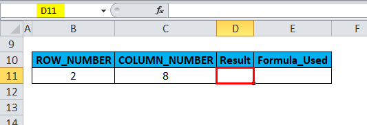
In the below-mentioned example, I have a row number in Cell “B11” & a column number in cell “C11”. Here I need to find the cell address with row & column numbers.
Let’s apply the ADDRESS function in cell “D11”. Select the cell “D11,” where the ADDRESS function needs to be applied.
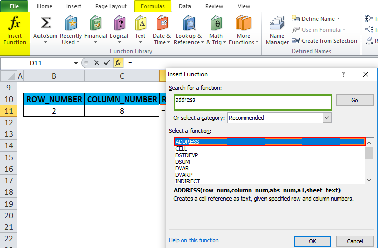
Click the insert function button (fx) under the formula toolbar, and a dialog box will appear, type the keyword “ADDRESS” in the search for a function box, and the ADDRESS function will appear in the select function box. Double click on the ADDRESS function.
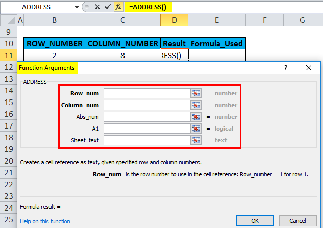
A dialog box appears where arguments for the ADDRESS function need to be filled or entered i.e.
=ADDRESS(row_num, column_num, [abs_num], [a1], [sheet_text])
- Row or row_num: (Compulsory or required parameter) It is a row number of the cell address. Here it is 2.
- Column or Column_num: (Compulsory or required parameter) It is a Column number of the cell address. Here it is, 8.
- [abs_num] or ref_type: (optional argument) This argument is omitted or not entered. By default, it will consider 1, i.e., Absolute reference.
- [ref_style] or [a1] : (optional argument) This argument is omitted or not entered. By default, it will consider 1 or TRUE (A1 style).
- [sheet_text]) or [sheet_name]: (optional argument) This argument is omitted or not entered; it is left blank. By default, no sheet name appears.
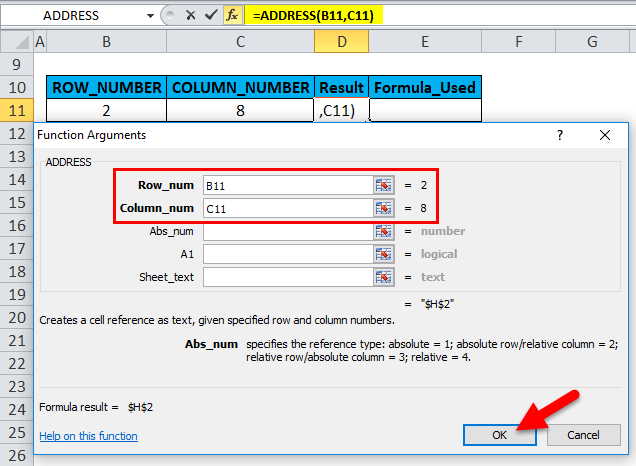
Click ok, after entering all the ADDRESS function arguments.
=ADDRESS(B11,C11) or =ADDRESS(2,8)
When the above parameters or arguments, i.e. ([abs_num], [a1], [sheet_text]), are not mentioned, then the ADDRESS function results in or returns a pattern of absolute address with row and column name (i.e., $H$2).
$H indicates the Absolut column (8), whereas $2 indicates the Absolute Row (2).
Example #2
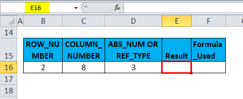
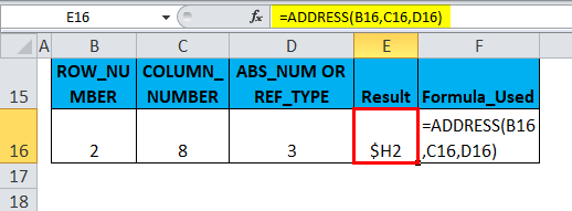
In the below-mentioned example, I have a row number in Cell “B16,” & a column number in cell “C8,” & Reference type or abs_num as 3 in cell “D16”. Here I need to find out the cell address & it should reflect as Absolute Column & Relative Row in Cell Address.
Let’s apply the ADDRESS function in cell “E16”. Select the cell “E16”. where the ADDRESS function needs to be applied.
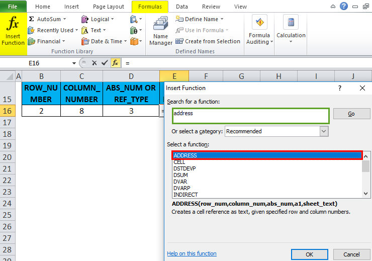
Click the insert function button (fx) under the formula toolbar, and a dialog box will appear, type the keyword “ADDRESS” in the search for a function box, ADDRESS function will appear in the select function box. Double click on the ADDRESS function.
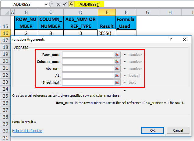
A dialog box appears where arguments for the ADDRESS function need to be filled or entered i.e.
=ADDRESS(row_num, column_num, [abs_num], [a1], [sheet_text])
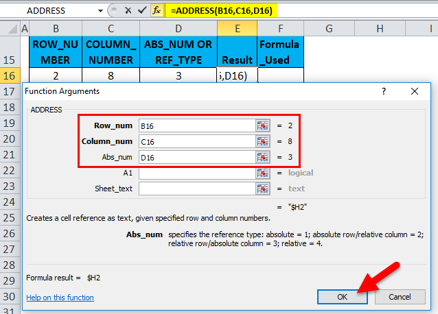
- Row or row_num: (Compulsory or required parameter) It is a row number of the cell address. Here it is 2.
- Column or Column_num: (Compulsory or required parameter) It is a column number of the cell address. Here it is, 8.
- [abs_num] or ref_type: (optional argument) Here, in the cell address, output is to be returned as an absolute column & relative row in cell address. Therefore, we have to enter 3.
- [ref_style] or [a1] : (optional argument) This argument is omitted or not entered. By default, it will consider 1 or TRUE (A1 style).
- [sheet_text]) or [sheet_name]: (optional argument) This argument is omitted or not entered. It is left blank. By default, no sheet name appears.
Click ok after entering all the ADDRESS function arguments. i.e.
=ADDRESS(2,8,3)
ADDRESS function results in or returns a pattern of absolute column & relative row in cell address (i.e., $H2).
Here, $H indicates the Absolut column, whereas 2 indicates the relative Row (2).
Things to Remember
#VALUE! error occurs if the row or column number argument is less than 1. If the Column number is greater than the number of columns in Excel (16,384 Columns). If the row number exceeds the number of rows in Excel (10,48,576 rows).
In the ADDRESS function argument, if row_num, column_num, or [abs_num] is a nonnumeric value, it returns #VALUE! Error.
Recommended Articles
This has been a guide to ADDRESS in Excel. Here we discuss the ADDRESS Formula in Excel and How to use the ADDRESS Function in Excel, along with practical examples and a downloadable Excel template. You can also go through our other suggested articles –


