Amortization Formula (Table of Contents)
Amortization Formula
Amortization is paying off debt amount periodically until the loan principal reduces to zero. The amount paid monthly is known as EMI, which is equated to monthly installments.
EMI has principal and interest components calculated by the amortization formula. Amortization calculation depends on the principal, the Rate of interest, and the time period of the loan. Amortization can be done manually or by Excel formula, for both are different.
Now, let us see how to calculate Amortization manually.
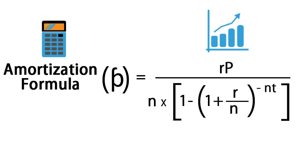
Monthly payment, i.e., can be calculated by the below formula:-
The formula for interest is as follows:-
Where,
- P = Principal
- r= Rate of interest
- t = Time in terms of year
- n = Monthly payment in a year
- I = Interest
- ƥ = Monthly Payment or EMI amount
Example of Amortization Formula
Now, let’s see an example to understand the calculation.
A salaried person took a home loan from a bank of $100,000 at the Rate of interest of 10% for a period of 20 years. Now, we must calculate the EMI amount and interest component paid to the bank.
- P = $100,000
- r= 10% i.e 0.1
- t = 20
- n = 12
Amortization is Calculated Using Below formula:
- ƥ = rP / n * [1-(1+r/n)-nt]
- ƥ = 0.1 * 100,000 / 12 * [1-(1+0.1/12)-12*20]
- ƥ = 965.0216
And now, to calculate interest paid, we will put value in the interest formula.
- I = nƥt – P
- I = 12*965.0216*20 – 100,000
- I = $131,605.2
So, the interest paid on the loan is $131,605.2.
Significance and Use of Amortization Formula
There are many uses of Amortization. They are as follows:-
- It helps the lender as well as the borrower with systematic repayment.
- There are significantly fewer chances of error.
- The borrower can check the principal amount outstanding at any point in Time.
- It creates transparency between the borrower and the lender.
Amortization is calculated for loan repayment. Amortization prepares personal, home, and Auto loan repayment schedules. It gives in-depth details from the beginning till the maturity of the loan. If any borrower makes the part payment, his amortization schedule changes, and the effect is visible on EMI or tenure. That means the borrower can request for tenure change where EMI tenure will reduce and his EMI amount will be the same, or he can request a change in EMI where his EMI amount will reduce and tenure will be the same. In loans, more prepayment is done will result in less interest as the principal balance will reduce. Calculation became very easy using Amortization, even in the above scenario.
Amortization Calculator
You can use the following Amortization Formula Calculator
| r | |
| P | |
| n | |
| t | |
| Amortization Formula = | |
| Amortization Formula = |
| |||||||||
|
Amortization Formula in Excel (With Excel Template)
Now, let us see how Excel can calculate Amortization.
A couple took an auto loan from a bank of $10,000 at the Rate of interest of 10% for a period of 2 years. Now, we have to calculate the EMI amount for the same.
Amortization in Excel is calculated using the below formula:
= PMT(Rate,nper,pv)
In Excel, one can use the below formula to calculate the amortization value:-
- For the calculation of interest paid during a specific period, we will use the below formula.
=ISPMT(Rate,per,nper,pv)
- To calculate the amount of payment in a period below formula is used.
= PMT(Rate,nper,pv)
- To calculate the number of payments below formula is used.
= NPER(Rate,pmt,pv)
- To calculate cumulative interest payment for periods n1 through n2.
=CUMIPMT(rate,nper,pv,n1,n2,0)
- To calculate the cumulative principal payment for periods n1 through n2.
=CUMIPRINC(rate,nper,pv,n1,n2,0)
- To calculate the principal paid in an EMI below formula is used.
=PPMT(rate,per,nper,pv)
Where
- pv = Present value of the loan
- pmt = Payment per period
- nper = Number of payment period
- rate = Rate of interest
Through the above formula repayment schedule for a loan over a period is prepared, which is known as an amortization schedule.
Below are steps to prepare an amortization schedule in Excel.
- Put input of formula in a standard format.
| Principal | $200,000 |
| Rate of Interest | 9% |
| Tenure(In years) | 10 |
- Plot table for an amortization schedule. In the zero month column, put the balance as $200,000 and then put 1, 2, 3, and so on till the last month of EMI in the month field.
| Month | EMI | Principal | Interest | Balance |
- Calculate EMI with the below formula:-
= PMT(Rate,nper,pv)
- Calculate the principal with the below formula:-
=PPMT(rate,per,nper,pv)
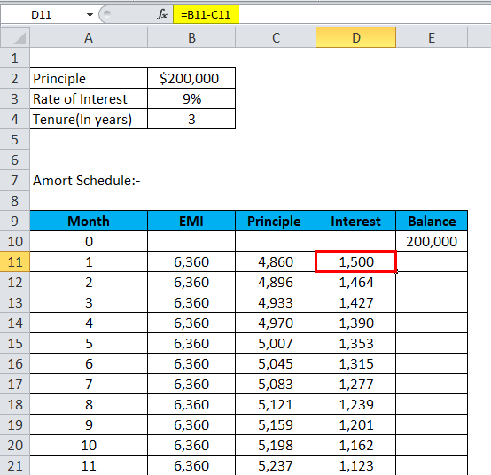
- Now, interest will be:-
Interest = EMI – Principal
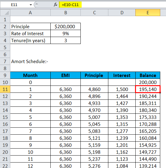
- The balance will be the previous balance minus the principal.
Balance = Previous Balance – Principal
- Repeat until last month, and we will get the amortization schedule.
Now, we will see an example of preparing an amortization schedule.
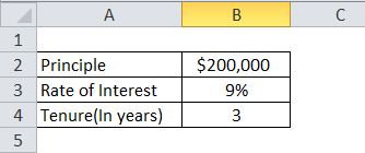
A person has taken an auto loan of $200,000 with a rate of interest of 9% for a tenure of 3 years and wants to prepare his amortization schedule.
Using the above formulas in Excel, he gets an amortization schedule.
- Put input of formula in a standard format.
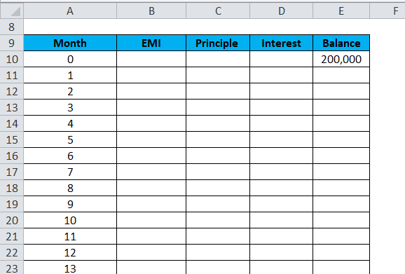
- Plot table for the amortization schedule. In the zero month column, put the balance as $200,000 and then put 1, 2, 3, and so on till the last month of EMI in the month field.
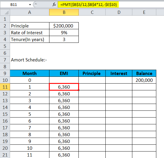
- Calculate EMI with the below formula:-
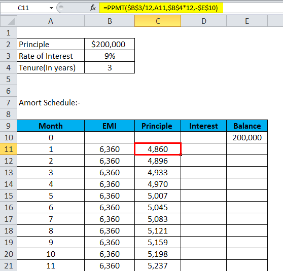
- Calculate the principal with the below formula:-
- Now, interest will be:-
- The balance will be the previous balance minus the principal.
- Repeat the same till last month, and he will get the below amortization schedule.
| Month | EMI | Principal | Interest | Balance |
| 0 | 200,000 | |||
| 1 | 6,360 | 4,860 | 1,500 | 195,140 |
| 2 | 6,360 | 4,896 | 1,464 | 190,244 |
| 3 | 6,360 | 4,933 | 1,427 | 185,311 |
| 4 | 6,360 | 4,970 | 1,390 | 180,340 |
| 5 | 6,360 | 5,007 | 1,353 | 175,333 |
| 6 | 6,360 | 5,045 | 1,315 | 170,288 |
| 7 | 6,360 | 5,083 | 1,277 | 165,205 |
| 8 | 6,360 | 5,121 | 1,239 | 160,084 |
| 9 | 6,360 | 5,159 | 1,201 | 154,925 |
| 10 | 6,360 | 5,198 | 1,162 | 149,727 |
| 11 | 6,360 | 5,237 | 1,123 | 144,490 |
| 12 | 6,360 | 5,276 | 1,084 | 139,214 |
| 13 | 6,360 | 5,316 | 1,044 | 133,898 |
| 14 | 6,360 | 5,356 | 1,004 | 128,542 |
| 15 | 6,360 | 5,396 | 964 | 123,146 |
| 16 | 6,360 | 5,436 | 924 | 117,710 |
| 17 | 6,360 | 5,477 | 883 | 112,233 |
| 18 | 6,360 | 5,518 | 842 | 106,715 |
| 19 | 6,360 | 5,560 | 800 | 101,155 |
| 20 | 6,360 | 5,601 | 759 | 95,554 |
| 21 | 6,360 | 5,643 | 717 | 89,911 |
| 22 | 6,360 | 5,686 | 674 | 84,225 |
| 23 | 6,360 | 5,728 | 632 | 78,497 |
| 24 | 6,360 | 5,771 | 589 | 72,725 |
| 25 | 6,360 | 5,815 | 545 | 66,911 |
| 26 | 6,360 | 5,858 | 502 | 61,053 |
| 27 | 6,360 | 5,902 | 458 | 55,151 |
| 28 | 6,360 | 5,946 | 414 | 49,204 |
| 29 | 6,360 | 5,991 | 369 | 43,214 |
| 30 | 6,360 | 6,036 | 324 | 37,178 |
| 31 | 6,360 | 6,081 | 279 | 31,097 |
| 32 | 6,360 | 6,127 | 233 | 24,970 |
| 33 | 6,360 | 6,173 | 187 | 18,797 |
| 34 | 6,360 | 6,219 | 141 | 12,578 |
| 35 | 6,360 | 6,266 | 94 | 6,313 |
| 36 | 6,360 | 6,313 | 47 | 0 |
Amortization Schedule
An amortization schedule helps one to know when they have to pay EMI against their loan and the EMI they need to pay, how much interest they have to pay on their loan, and what is the principal outstanding of the loan. It is a very systematic and easy way to track loan repayment.
Amortization ends when the loan matures, and the principal balance is zero. Suppose the amount is not recovered from the borrower. In that case, the interest accrued will be added to the outstanding amount, which leads to an increase in the principal of the loan, known as negative Amortization.
Recommended Articles
This has been a guide to an Amortization formula. Here we discuss its uses along with practical examples. We also provide you with an Amortization Calculator with a downloadable Excel template. You may also look at the following articles to learn more –


