What is Analyzing Time Series Data
Time series data is a collection of data points gathered, observed, or documented at regular intervals. Each data point is linked to a specific timestamp or time period. This data type is widely utilized in finance, economics, weather forecasting, and signal processing to examine trends, patterns, and changes over time and forecast future behavior based on past observations.
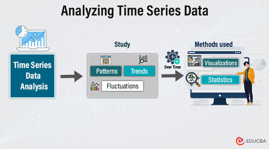
Table of Contents
Key Takeaways
- Pattern Identification: Time series analysis identifies trends, seasonal variations, and anomalies, providing crucial insights.
- Predictive Power: By analyzing data, organizations can forecast future trends, aiding proactive decision-making.
- Technique Utilization: Organizations commonly use moving averages and ARIMA models to analyze trends and make predictions.
- Strategic Impact: Insights from time series data enhance business planning and risk management, ensuring organizational resilience.
How to Analyze Time Series?
To perform time series analysis effectively, the following steps are typically followed:
Data Collection and Cleansing:
- Acquire time series data from reputable sources, ensuring its accuracy and completeness.
- To uphold data integrity, refine the data by addressing missing values, outliers, and inconsistencies.
Preparing Visualization with Time vs Key Feature:
- Graph the time series data against the relevant time periods to represent trends and patterns visually.
- Identify pivotal features or variables and depict their behavior and relationships over time.
Observing Stationarity:
- Evaluate the time series data for stationarity, indicating that statistical properties such as mean and variance remain constant over time.
- Utilize methods such as rolling statistics, the Augmented Dickey-Fuller (ADF) test, or visual examination of plots to gauge stationarity.
Utilizing Charts for Enhanced Understanding of Natural Phenomena:
- Generate supplementary charts and graphs further to analyze the characteristics of the time series data.
- Investigate seasonal decomposition, autocorrelation, and partial autocorrelation plots to identify seasonal patterns and correlations.
Constructing Models – AR, MA, ARMA, and ARIMA:
- Select suitable time series models based on the observed data characteristics.
- AR (AutoRegressive) models capture the relationship between an observation and several lagged observations.
- MA (Moving Average) models depict the relationship between an observation and the residual error from a moving average model.
- ARMA (AutoRegressive Moving Average) models combine AR and MA components.
- ARIMA (AutoRegressive Integrated Moving Average) models incorporate differencing to make the time series stationary before modeling.
Deriving Insights from Forecasts
- Utilize the established models to forecast future values of the time series.
- Assess the precision of the forecasts using suitable metrics and portray the forecasted values alongside the actual values.
- Derive meaningful insights from the forecasts to guide decision-making and comprehend the potential impact on future trends or behaviors.
Why organizations use time series data analysis
Organizations use time series data analysis for several reasons:
- Forecasting and Prediction: Time series analysis assists organizations in projecting future trends, behaviors, and events based on historical data. It facilitates improved planning, resource allocation, and decision-making.
- Performance Monitoring: By analyzing time series data, organizations can evaluate the performance of various metrics and key performance indicators (KPIs) over time. It empowers them to pinpoint trends, anomalies, and areas for enhancement.
- Risk Management: Time series analysis helps organizations identify and assess risks by scrutinizing historical patterns and predicting potential risks. It facilitates proactive risk mitigation strategies and contingency planning.
- Demand Planning and Inventory Management: Time series analysis aids organizations in projecting product or service demand, optimizing stock levels, and enhancing supply chain management efficiency.
- Financial Analysis: Within finance, time series analysis plays a critical role in evaluating stock prices, market trends, and economic indicators. It enables organizations to make well-informed investment decisions, manage portfolios, and assess financial risk.
- Analysis of Customer Behavior: Utilizing time series analysis allows organizations to examine customer behavior longitudinally, encompassing purchasing trends, website visitation, and engagement metrics. It facilitates the customization of marketing strategies, the enhancement of customer retention efforts, and the improvement of overall customer experience.
Characteristics of Time Series Data
- Temporal Ordering: Data points are arranged in order of occurrence, with each observation linked to a specific point in time or time span.
- Seasonality: Numerous time series display repetitive patterns or cycles at regular intervals, including daily, weekly, monthly, or yearly fluctuations.
- Trend: Time series data frequently showcases a prolonged trend, indicating an overall upward or downward progression over time. Trends may manifest as linear, exponential, or nonlinear patterns.
- Variability: Time series data may demonstrate variations or fluctuations around the underlying trend, encompassing random noise, irregular patterns, or volatility.
- Autocorrelation: Within a time series, there may be a correlation between current and previous observations at various time lags, suggesting interdependencies or connections between consecutive data points.
- Stationarity: Stationarity pertains to the constancy of statistical characteristics over time, encompassing steady mean, variance, and autocovariance. Numerous time series models rely on stationarity for precise forecasting.
- Irregular Events: Time series data could encompass irregular events or outliers, representing unforeseen incidents or anomalies that diverge from typical patterns.
- Periodicity: Certain time series display periodic patterns, where behaviors recur at consistent intervals, such as seasonal variations in sales or temperature.
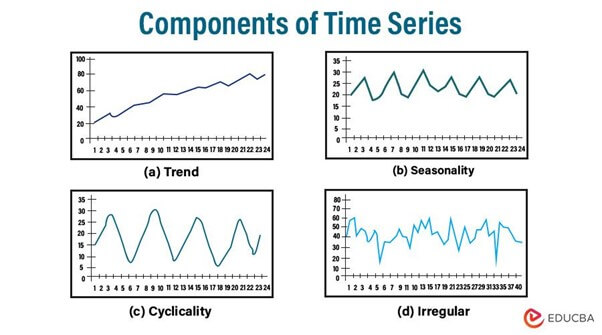
Components of Time Series Data
- Trend
The trend component signifies the extended movement or directionality observed in the data over time. It captures the fundamental pattern that indicates whether the series is generally increasing, decreasing, or remaining stable. Trends can manifest as linear, following a straight line, or nonlinear, displaying more intricate patterns such as exponential growth or decay. Understanding the trend assists analysts in recognizing overall patterns and forecasting future behavior. Factors such as economic conditions, technological advancements, population growth, or changes in consumer behavior can influence trends.
- Seasonality
The trend component signifies the extended movement or directionality observed in the data over time. It captures the fundamental pattern that indicates whether the series is generally increasing, decreasing, or remaining stable. Trends can manifest as linear, following a straight line, or nonlinear, displaying more intricate patterns such as exponential growth or decay. Understanding the trend assists analysts in recognizing overall patterns and forecasting future behavior. Factors such as economic conditions, technological advancements, population growth, or changes in consumer behavior can influence trends.
- Cyclical Trends
Cyclical patterns signify oscillations or data fluctuations taking place over periods longer than seasonal patterns. Unlike seasonality, cyclical patterns lack fixed frequencies or durations and may display irregular or variable lengths. These variations are often linked with economic cycles, including periods of business activity expansion and contraction or long-term market condition trends. Identifying cyclical patterns aids analysts in comprehending broader economic trends and predicting potential turning points or phases in the business cycle.
- Irregularity:
The irregularity, or residual component, denotes the stochastic fluctuations or noise in the data that cannot be attributed to the underlying trend, seasonality, or cyclic patterns. It encompasses the unforeseeable variations or interferences within the time series. Irregularities may stem from factors such as measurement inaccuracies, one-time occurrences, or unexpected disruptions in the data-generating process. Even though irregularities may lack a discernible pattern, they can still impact the precision of forecasting models, and analysts should consider them in the analysis.
Types of Time Series Data
- Univariate Time Series
- Univariate time series data is collected by observing a single variable over a period of time.
- It illustrates the progression of a singular phenomenon or measurement, for instance, stock prices, temperature recordings, or sales figures.
- The examination of univariate time series centers on comprehending the patterns, seasonality, and anomalies evident in the data.
- Multivariate Time Series
- Multivariate temporal data refers to the simultaneous observation of multiple variables over time.
- It encompasses the interconnections and interdependencies among various phenomena or measurements, enabling more intricate analysis.
- Instances encompass economic metrics such as GDP, inflation, and unemployment rates, with each variable exerting influence on the others.
- Longitudinal Time Series:
- Longitudinal time series data tracks the evolution of multiple individuals or entities over time.
- It is commonly used in longitudinal studies or panel data analysis to study trends and changes in individuals’ characteristics or behaviors over time.
- Examples include tracking students’ academic performance over multiple years or monitoring the health outcomes of patients in a clinical trial.
- Time-Series Panel Data
- Time-series panel data integrates cross-sectional and time-series elements, capturing observations from various entities at different time intervals.
- It facilitates the examination of variations within and between entities over time.
- Time-series panel data frequently finds application in econometrics, social sciences, and market research for analyzing the evolution of individual entities over time and their inter-entity distinctions.
- Time Series at High Frequencies:
- Time series at high frequencies capture observations at brief intervals, such as seconds, minutes, or hours.
- This data type is frequently leveraged in financial markets to study intraday price dynamics or in sensor data analysis to monitor physical systems in real time.
- Given its substantial volume and swift rate of change, managing high-frequency data presents challenges concerning data storage, processing, and modeling.
Preprocessing Time Series Data
Preprocessing time series data is essential before analyzing or utilizing it for machine learning purposes. The following are critical steps involved:
- Data Cleaning and Inspection:
- Handling Missing Values: Determine and manage missing values through techniques such as imputation, interpolation, or removal, taking into consideration the severity and context.
- Outliers: Identify and manage outliers using methods such as capping, winsorizing, or removal, based on the level of severity and domain expertise.
- Time Consistency: Verify consistent timestamps and data collection frequency and address duplicates or gaps in timestamps.
- Stationarity: Analyze and adjust series to achieve stationarity if necessary for further analysis, using techniques like differencing, trend removal, or transformation.
- Feature Engineering:
- Lag features: Generate historical versions of the target variable to incorporate past data.
- External factors: Integrate pertinent external elements that could impact the series.
- Context-specific features: Develop features based on the particular domain and problem context.
- Normalization of features: Standardize or normalize features to mitigate issues with algorithms sensitive to scale.
- Transformation:
- Logarithmic transformation: Useful for data with skewed distributions or large variations.
- Offsetting: Employed to attain stationarity by eliminating trends or seasonality.
- Spectral decomposition: Breaks down the series into trend, seasonality, and noise constituents.
- Dimensionality Reduction:
- Principal Component Analysis (PCA): Diminishes data dimensionality while retaining the highest variance.
- Time series clustering: Aggregates analogous time series for additional analysis.
- Data Splitting:
- Train-Test Split: Segregate data into training and testing subsets to facilitate model development and assessment.
- Validation Set: Optionally, employ a distinct validation set to refine
Time Series Visualization
Time series visualization is critical in analyzing time-dependent data, including stock prices, temperature readings, sales figures, etc. These visualizations are instrumental in gaining valuable insights, uncovering patterns, and facilitating informed decision-making. This underscores the significance of time series visualization and the diverse contributions that various types of graphs offer.
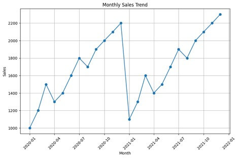
Let’s use a hypothetical example of monthly sales data for a retail store to demonstrate various time series visualizations. Suppose we have the following monthly sales data for the past two years:
- Line Plots:
- Functionality: Line plots are the most basic type of time series visualization that displays the trend of a variable over time.
- Purpose: They help to visualize the overall trend, direction, and magnitude of change in the data over the specified time period.
- Usage: Line plots are useful for identifying long-term trends, detecting abrupt changes, and comparing multiple time series.
Libraries
import pandas as pd
import matplotlib.pyplot as plt
import seaborn as sns
Monthly Sales Dataset
# Define the monthly sales data
data = {
    'Month': ['Jan 2020', 'Feb 2020', 'Mar 2020', 'Apr 2020', 'May 2020', 'Jun 2020', 'Jul 2020', 'Aug 2020', 'Sep 2020', 'Oct 2020', 'Nov 2020', 'Dec 2020',
              'Jan 2021', 'Feb 2021', 'Mar 2021', 'Apr 2021', 'May 2021', 'Jun 2021', 'Jul 2021', 'Aug 2021', 'Sep 2021', 'Oct 2021', 'Nov 2021', 'Dec 2021'],
    'Sales': [1000, 1200, 1500, 1300, 1400, 1600, 1800, 1700, 1900, 2000, 2100, 2200,
              1100, 1300, 1600, 1400, 1500, 1700, 1900, 1800, 2000, 2100, 2200, 2300]
}
# Create DataFrame
df = pd.DataFrame(data)
# Convert Month column to datetime
df['Month'] = pd.to_datetime(df['Month'])
# Line Plot
plt.figure(figsize=(10, 6))
plt.plot(df['Month'], df['Sales'], marker='o', linestyle='-')
plt.title('Monthly Sales Trend')
plt.xlabel('Month')
plt.ylabel('Sales')
plt.xticks(rotation=45)
plt.grid(True)
plt.show()- Seasonal Subseries Plots:
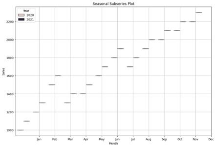
- Functionality: Seasonal subseries plots partition the time series data into seasons (e.g., months) and display each season’s values separately.
- Purpose: They help to visualize the seasonal pattern or cyclicality within each year by providing a clearer view of the seasonal variation.
- Usage: Seasonal subseries plots are useful for detecting seasonal effects, identifying any systematic patterns within each season, and comparing seasonal behavior across different years.
# Seasonal Subseries Plot
plt.figure(figsize=(12, 8))
sns.boxplot(x=df['Month'].dt.month, y=df['Sales'], hue=df['Month'].dt.year)
plt.title('Seasonal Subseries Plot')
plt.xlabel('Month')
plt.ylabel('Sales')
plt.xticks(ticks=range(1, 13), labels=['Jan', 'Feb', 'Mar', 'Apr', 'May', 'Jun', 'Jul', 'Aug', 'Sep', 'Oct', 'Nov', 'Dec'])
plt.legend(title='Year')
plt.grid(True)
plt.show()- Boxplots:
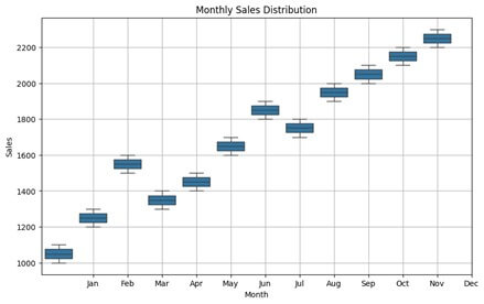
- Functionality: Boxplots display the distribution of a numeric variable (e.g., sales) across different categories (e.g., months or seasons).
- Purpose: They help to identify outliers, variations, and the spread of the data within each category.
- Usage: Boxplots are useful for detecting anomalies, comparing distributions across different categories, and assessing the variability of the data.
# Boxplot
plt.figure(figsize=(10, 6))
sns.boxplot(x=df['Month'].dt.month, y=df['Sales'])
plt.title('Monthly Sales Distribution')
plt.xlabel('Month')
plt.ylabel('Sales')
plt.xticks(ticks=range(1, 13), labels=['Jan', 'Feb', 'Mar', 'Apr', 'May', 'Jun', 'Jul', 'Aug', 'Sep', 'Oct', 'Nov', 'Dec'])
plt.grid(True)
plt.show()- Autocorrelation Plots:
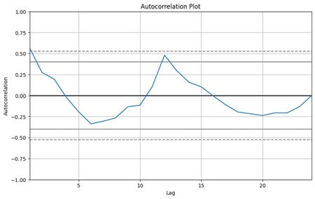
- Functionality: Autocorrelation plots show the correlation between a time series and its lagged values (i.e., values from previous time periods).
- Purpose: They help to identify any correlation or dependency between the current value of the series and its past values.
- Usage: Autocorrelation plots are useful for detecting seasonality, trend, or other patterns that depend on the series’ own past values.
# Autocorrelation Plot
plt.figure(figsize=(10, 6))
pd.plotting.autocorrelation_plot(df['Sales'])
plt.title('Autocorrelation Plot')
plt.xlabel('Lag')
plt.ylabel('Autocorrelation')
plt.grid(True)
plt.show()- Heatmaps:
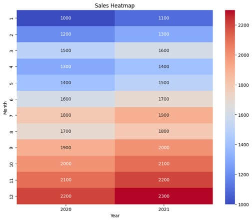
- Functionality: Heatmaps visualize the correlation matrix between multiple variables (e.g., sales for each month) using colors to represent the strength and direction of the correlation.
- Purpose: They help to identify relationships, patterns, and dependencies between variables.
- Usage: Heatmaps are useful for exploring complex relationships, identifying clusters or groups of variables, and understanding the overall structure of the data.
# Heatmap
plt.figure(figsize=(10, 8))
correlation_matrix = df.pivot_table(values='Sales', index=df['Month'].dt.month, columns=df['Month'].dt.year, aggfunc='mean')
sns.heatmap(correlation_matrix, cmap='coolwarm', annot=True, fmt='.0f')
plt.title('Sales Heatmap')
plt.xlabel('Year')
plt.ylabel('Month')
plt.show()Cross-Sectional Data Vs. Time Series Data
| Section | Cross-Sectional Data | Time Series Data |
| Definition | Data collected at a single point in time | Data collected over multiple time periods |
| Observation Units | Different entities or individuals | Same entity or individual over time |
| Examples | Survey responses, census data | Stock prices, temperature readings |
| Dimensionality | Two-dimensional | Two-dimensional |
| Analysis Focus | Comparing different entities at a specific time | Analyzing trends and patterns over time |
| Statistical Tests | T-tests, ANOVA, chi-square tests | Autocorrelation, time series decomposition |
| Visualization | Bar charts, scatter plots | Line graphs, time series plots |
| Forecasting | Not applicable | Time series forecasting models |
Challenges and Best Practices
Analyzing time series data presents a unique set of challenges stemming from the temporal nature and inherent characteristics of the data. The following outlines common challenges and best practices for analyzing time series data.
Challenges:
- Temporal Dependencies: Time series data frequently displays intricate temporal interrelationships, encompassing trends, seasonality, and autocorrelation. Accurately capturing and modeling these interdependencies is pivotal for conducting effective analysis.
- Noise and Outliers: Time series data may contain irregular fluctuations and outliers, leading to noisy fluctuations. Appropriately identifying and addressing noise and outliers is critical to prevent misinterpreted analysis results.
- Non-Stationarity: Many time series demonstrate non-stationary behavior, indicating that statistical characteristics such as mean and variance evolve over time. Effectively handling non-stationarity necessitates meticulous preprocessing and modeling techniques.
- Missing Data: Time series data may contain gaps due to factors such as sensor malfunctions, data collection inaccuracies, or incomplete records. Effectively managing missing data and imputing values without bias is critical to time series analysis.
- Complexity of Models: Selecting an appropriate model for time series analysis can be daunting due to the wide array of available models and their intricacies. It is crucial to identify a model that strikes a balance between accuracy and interpretability.
- Forecasting Uncertainty: Time series forecasting entails predicting future values while also estimating the uncertainty associated with the predictions. Effectively capturing and quantifying uncertainty is essential for creating reliable forecasts and making informed decisions.
Best Practices:
- Data Preprocessing: Thorough data preprocessing is imperative for analyzing time series. This encompasses addressing missing values, detrending, deseasonalizing, and standardizing the data to render it suitable for modeling.
- Exploratory Data Analysis (EDA): Conducting exploratory data analysis aids in comprehending the underlying patterns, trends, and seasonality within the data. Visualization techniques, such as time series, autocorrelation, and decomposition plots, can yield valuable insights.
- Model Selection: The selection of appropriate models hinges upon the characteristics of the data and the specific analysis objectives. Factors such as stationarity, seasonality, autocorrelation, and data complexity should be considered when selecting models.
- Cross-Validation: Utilize methodologies like cross-validation to appraise the efficacy of time series models and prevent overfitting. Segment the data into training and validation sets to assess the model’s performance on unseen data.
- Ensemble Methods: Integrate predictions from multiple models using ensemble methods such as averaging, stacking, or boosting to enhance prediction accuracy and resilience.
- Continuous Monitoring: Regularly monitor and adjust time series models to adapt to evolving data patterns and ensure their sustained precision and efficacy.
- Documentation and Analysis: Record the complete analysis process, encompassing data preprocessing procedures, model selection considerations, and assessment metrics. Explain the outcomes within the framework of the problem domain and effectively convey findings to stakeholders.
Conclusion
The time series data analysis reveals patterns and trends crucial for informed decision-making. This analysis empowers stakeholders to optimize strategies and resource allocation by identifying correlations and forecasting future outcomes. Understanding temporal dynamics enhances predictive accuracy and fosters adaptability in dynamic environments, driving sustainable growth and efficiency.
Frequently Asked Questions (FAQs)
Q1. What is stationarity in time series analysis?
Answer: Stationarity refers to the statistical properties of a time series that remain constant over time. A stationary time series exhibits constant mean, constant variance, and autocovariance that does not depend on time. Stationarity is often a prerequisite for many time series modeling techniques.
Q2. What software tools are commonly used for time series analysis?
Answer: Popular software tools for time series analysis include Python libraries like pandas, NumPy, statsmodels, and scikit-learn, as well as R programming language with packages like forecast, TSA, and zoo. Additionally, specialized software such as MATLAB, SAS, and STATA also offer time series analysis capabilities.
Q3. Can I apply time series analysis to non-uniformly sampled data?
Answer: Yes, time series analysis techniques can be adapted for non-uniformly sampled data using methods like interpolation, resampling to a regular grid, or employing specialized algorithms designed for irregularly spaced time series, such as Gaussian process regression or time warping techniques.
Q4. What are some common applications of time series analysis?
Answer: Time series analysis is widely used in various fields such as finance (stock market forecasting), economics (GDP analysis), weather forecasting, signal processing, and many others. It’s particularly useful when understanding trends, making forecasts, or detecting anomalies over time.
Recommended Articles
We hope that this EDUCBA information on “Time Series Forecasting Models” was beneficial to you. You can view EDUCBA’s recommended articles for more information.
