Introduction to Backward Elimination
As man and machine knocking towards digital evolution, diverse technique machines are accounting to get themselves not only trained but smartly trained to come out with better recognition of real-world objects. Such a technique introduced earlier called “Backward Elimination” that intended to favor indispensable features while eradicating nugatory features to indulge better optimization in a machine. The entire proficiency of object recognition by Machine is proportionate to what features it considering.
Features that have no reference on the predicted output must be discharged out from the machine and it is concluded by backward elimination. Good Precision and time complexity of recognition of any real word object by Machine depend on its learning. So backward eliminate plays its rigid role for feature selection. It reckons the rate of dependency of features to the dependent variable finds the significance of its belonging in the model. To accredit this, it checks the reckoned rate with a standard significance level (say 0.06) and takes a decision for feature selection.
Why Do We Entail Backward Elimination?
Unessential and redundant traits propel the complexity of machine logic. It devours time and model’s resources unnecessarily. So the Aforementioned technique plays a competent role to forge the model to simple. The algorithm cultivates the best version of the model by optimizing its performance and truncating its expendable appointed resources.
It curtails the least noteworthy features from the model which causes noise in deciding the line of regression. Irrelevant object traits may engender to misclassification and prediction. Irrelevant features of an entity may constitute a misbalance in the model with respect to other significant features of other objects. The backward elimination fosters the fitting of the model to the best case. Hence, backward elimination is recommended to use in a model.
How to Apply Backward Elimination?
The backward elimination commences with all feature variables, testing it with the dependent variable under a selected fitting of model criterion. It starts eradicating those variables which deteriorate the fitting line of regression. Repeating this deletion until the model attains a good fit. Below are the steps to practice the backward elimination:
Step 1: Choose the appropriate level of significance to reside in the model of the machine. (Take S=0.06)
Step 2: Fed all the available independent variables to the model with respect to the dependent variable and computer the slope and intercept to draw a line of regression or fitting line.
Step 3: Traverse with all the independent variable which possess the highest value (Take I) one by one and proceed with the following toast:-
a) If I > S, execute the 4th step.
b) Else abort and the model is perfect.
Step 4: Remove that chosen variable and increment the traversal.
Step 5: Re-forge the model again and compute the slope and intercept of the fitting line again with residual variables.
The aforementioned steps are summarized into the rejection of those features whose significance rate is above to the selected significance value (0.06) to evade over-classification and overutilization of resources which observed as high complexity.
Merits and Demerits of Backward Elimination
Here are some merits and demerits of backward elimination given below in detail:
1. Merits
Merits of backward elimination are as follows:
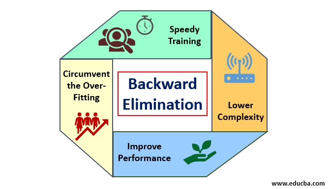
- Speedy Training: The machine is trained with a set of available features of pattern which is done in a very short time if unessential features are removed from the model. Speedy training of data set comes into picture only when the model is dealing with significant features and excluding all the noise variables. It draws a simple complexity for training. But the model should not undergo under-fitting which occurs due to lack of features or inadequate samples. The sample feature should be plentiful in a model for the best classification. The time requires to train the model should be less while maintaining classification accuracy and left with no under-prediction variable.
- Lower Complexity: The complexity of the model happens to be high if the model contemplates the extent of features including noise and unrelated features. The model consumes much space and time to process such a span of features. This may increase the rate of accuracy of pattern recognition, but the rate may contain noise as well. To get rid of such a high complexity of the model, the backward elimination algorithm plays a requisite role by retrenching the unwanted features from the model. It simplifies the processing logic of the model. Only a few essential features are ample to draw a good fit which contenting reasonable accuracy.
- Improve Performance: The model performance depends on many aspects. The model undergoes optimization by using backward elimination. The optimization of the model is the optimization of the dataset used for training the model. The model’s performance is directly proportional to its rate of optimization which relies on the frequency of significant data. The backward elimination process is not intended to starts alteration from any low-frequency predicator. But it only starts alteration from high-frequency data because mostly the model’s complexity depends over that part.
- Circumvent the Over-Fitting: The over-fitting situation occurs when the model got too many datasets and classification or prediction is conducted in which some predicators got the noise of other classes. In this fitting, the model supposed to give unexpectedly high accuracy. In over-fitting, the model may fail to classify the variable because of confusion created in logic due to too many conditions. The backward elimination technique curtails out the extraneous feature to circumvent the situation of over-fitting.
2. Demerits
Demerits of backward elimination are as follows:
- In the backward elimination method, one cannot find out which predicator is responsible for the rejection of another predicator due to its reaching to insignificance. For instance, if predicator X has some significance which was good enough to reside in a model after adding the Y predicator. But the significance of X gets outdated when another predicator Z comes into the model. So the backward elimination algorithm does not evident about any dependency between two predictors which happen in the “Forward selection technique”.
- After discarding any feature from a model by a backward elimination algorithm, that feature cannot be selected again. In short, backward elimination does not have a flexible approach to add or remove features/predictors.
- The norms to select the significance value (0.06) in the model are inflexible. The backward elimination does not have a flexible procedure to not only choose but also change the insignificant value as required in order to fetch the best fit under an adequate dataset.
Conclusion
The Backward elimination technique realized to ameliorate the model’s performance and to optimize its complexity. It vividly used in multiple regressions where the model deals with the extensive dataset. It is an easy and simple approach as compare to forward selection and cross-validation in which overload of optimization encountered. The backward elimination technique initiates the elimination of features of higher significance value. Its basic objective is to make the model less complex and forbid over-fitting situation.
Recommended Articles
This is a guide to Backward Elimination. Here we discuss how to apply backward elimination along with the merits and demerits. You may also look at the following articles to learn more-


