Updated August 21, 2023
Calculate Compound Interest in Excel
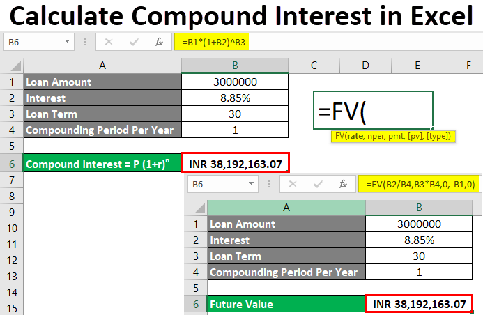
Compound Interest is the interest amount payable at a fixed interest rate for any fixed/variable term of investment/loan period on borrowed loan or invested amount. We can calculate the Compound Interest in Excel if we know the mathematical expression of it. A mathematical expression that we have already learned in school, Compound Interest, is shown below.
Where,
- P = Invested or Borrowed amount
- r = Yearly rate of Interest
- n = Invested or Loan term
How to Calculate Compound Interest in Excel?
To calculate compound interest in Excel is very simple and easy. Let’s understand how to calculate with some examples.
Excel Calculate Compound Interest – Example #1
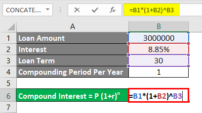
We have data on borrowed loan detail from any bank. For example, a person has borrowed a loan of Rs. 3000000/- from a bank with an annual interest rate of 8.85% for 30 Years. Detailed data is shown below.
Mostly compounding is done yearly. But it may vary from bank to bank and the type of investment is being done. In this case, we are considering the Compounding Period as 1.
Now let’s consider the mathematical formula for Excel calculating Compound Interest, which we have seen above.
Compound Interest = P (1+r)n
If we frame the formula with the above-mentioned value, then,
P = Rs. 3000000/-
r = 8.85%
n = 30 Years
For calculating compound interest, go to the cell where we want to see the output and type the “=” sign. And assign the above-mentioned value in a sequence of Compound Interest formulas in Excel, as shown below.
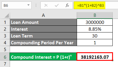
Here we have framed Compound interest; now press the Enter key to see the result.
As we can see, we have tallied our calculated compound interest. Rs.38192163.07/-. For 30 years, the person who borrowed the loan from the bank will be liable to pay Rs.38192163.07/- of compound interest.
We can assign the currency to calculate compound interest in Excel. For this, go to that cell and press Ctrl+1 or right-click to select Format Cells.
Format Cells dialog box will open. Go to Number and from there, under the category of Accounting.
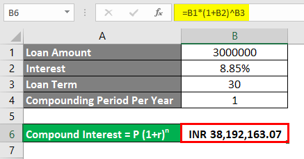
Select any applicable currency from the Symbol dropdown. Here we have selected INR (Indian Rupees). After that, click on Ok, as shown in the below screenshot.
As we can see, our calculated compound interest is showing the currency INR in the below screenshot.
Excel Calculate Compound Interest – Example #2
There is another method by which we can Calculate Compound Interest for any borrowed loan or invested amount. For this, we have considered the same data set that we have seen in Example-1.
Microsoft Excel has an inbuilt function named FV or Future Value, by which we can calculate the future value in terms of Compound Interest, Applicable loan with interest, and monthly EMI with one formula. To access the FV function, we can go to Insert Function beside the formula bar or type the “=” sign where we need to see the result. It will enable all the inbuilt functions of Excel. Now search and select FV from there, as shown below.
Where
- rate = Rate of interest,
- nper = Number of payments to be made. It can be monthly or years,
- pmt = fixed amount which needs to be paid monthly or yearly,
- pv = Present value of borrowed or invested amount (Optional),
- type = Use 1 if the EMI is paid at the start of the month, 0 if the EMI is paid at the end of the month. In Excel, automatically, it will consider as 0 (Optional).
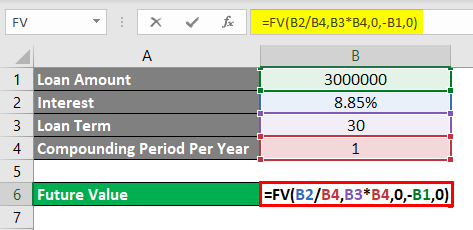
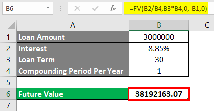
Now let’s frame the values in the above syntax of FV.
As we can see, we have considered the rate per compounding basis. So we have divided the 8.85% interest rate with compounding period 1 and multiplied nper, which is 30 with compounding period 1.
Once we select all the required parameters and complete our syntax, press the Enter key to see the result.
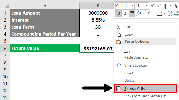
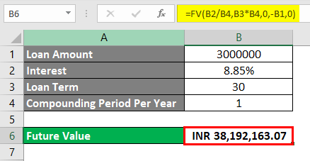
As we can see, the calculated compound interest as 38192163.07/- is without currency. We can add the required currency with the process seen in Example-1. For that, go to Format Cells or press Ctrl+1.
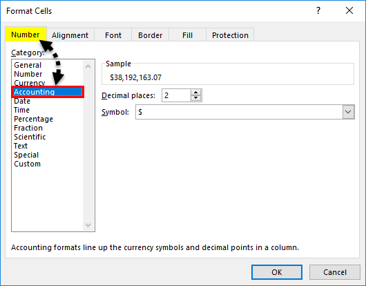
Format Cells dialog box pops up. Go to Number and from there, under the category of Accounting.
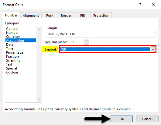
Select any applicable currency from the Symbol dropdown. Here we have selected INR (Indian Rupees). After that, click on Ok, as shown in the below screenshot.
We will get the selected currency as shown below.
Pros
- Compound interest is easy to calculate and calculate the values in Excel’s mathematical syntax.
- For real-life cases, we can easily calculate the interest payable on any loan or investment.
- We can use any of the mentioned methods for calculating compound interest for banking purposes.
Cons
- Compound interest is difficult to understand when and where to put a minus (“-“) sign before PV in syntax.
Things to Remember
- Calculating the compound interest with the formula and comparing the outcome is better. So that comparison can be made between the two outcomes.
- It is recommended to change/insert/update the currency to understand regional scenarios better.
- Understand the cases where we must put a minus sign before PV if we calculate compound interest from FV. Adding a minus sign indicates that we are liable to pay the amount to the bank. And plus sign shows the profit gained by the investor.
Recommended Articles
This is a guide to Calculate Compound Interest in Excel. Here we discuss how to calculate compound interest in Excel, along with practical examples and a downloadable Excel template. You can also go through our other suggested articles –

