Updated August 16, 2023
CEILING Function (Table of Contents)
Introduction to CEILING in Excel
The ceiling function is another mathematical function in Excel that is quite useful and is used for rounding off any decimal number closer to the value selected in the function but away from 0. RND function rounds off any decimal value to a whole number, whereas in the Ceiling function, we can choose the number to which extent we want to see the decimal number. We can either get the whole number or value in 0.5 formats.
In simple terms, you provide both number and significance numbers and ask Excel to round up the given to the nearest multiple of the given significance number.
For example: If the formula reads =CEILING (22, 8), it will return the value of 24. Now, let us break down the formula.
If you multiply 8 by 3, the resulting number is 24. The supplied number is 22, and the nearest multiple numbers of 8.
8 * 1 = 8 (Not nearest to 22)
8 * 2 = 16 (Not nearest to 22)
8 * 3 =24 (Nearest to 22)
8 * 4 = 32 (Too far from 22)
So CEILING function returns the nearest multiple of the significant number to the nearest supplied number.
CEILING Formula in Excel:
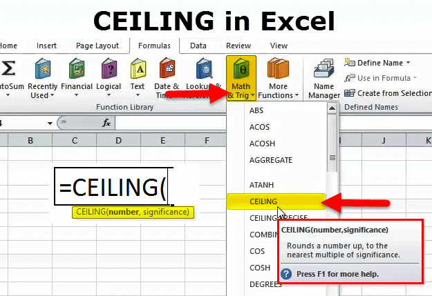
The Formula for the CEILING function is as follows:
The Formula of the CEILING function includes 2 arguments.
- Number: It is a mandatory argument. The number you want to round up.
- Significance: This is also a required argument. This is the number you are multiplying to round up the first given number.
How to Use the CEILING Function in Excel?
CEILING in Excel is very simple and easy to use. Let us understand the working of the CEILING function by some examples.
Example 1
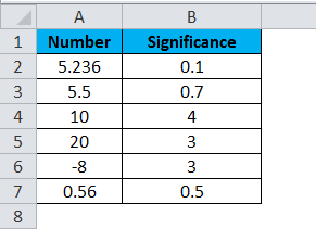
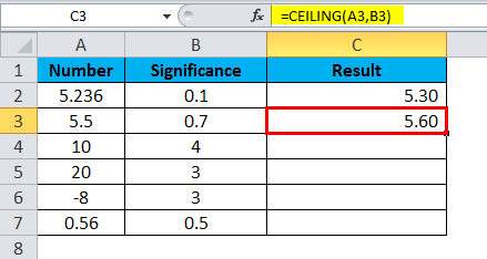
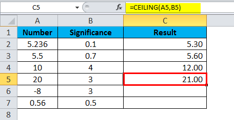
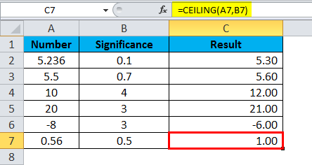
In the below image, I have applied the CEILING function to the numbers from A2:A7. I will discuss this one by one.
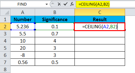
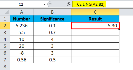
- In the first formula, the given number is 5.236, and the significance we are giving is 0.1. Formula used is =CEILING(A2,B2)
The formula returned the value of 5.3, which means the formula rounded up the 5.236 to the next nearest multiple of 0.1, i.e. 5.30.
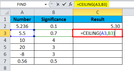
- In the second formula, we are rounding up the 5.5 to the next decimal number, i.e. 5.6. The formula used is =CEILING(A3,B3)
The significance we have given is 0.7, i.e. 0.7*8=5.60.
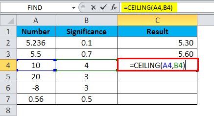
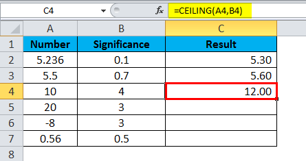
- Now look at the third formula number is 10, and the significant number is 4. One thing you need to observe here is 4*2=8 (this is also nearest to 10) and 4*3=12 (this is also nearest to 10). The formula used is =CEILING(A4,B4)
CEILING always returns the next nearest number. O, the result of the formula is 12.
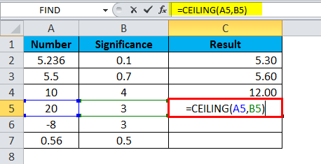
- The fourth formula number is 20, and the significant number is 3, i.e. 3*7 = 21, which is nearest to 20. Formula used is =CEILING(A5,B5)
The result of the formula is 21.
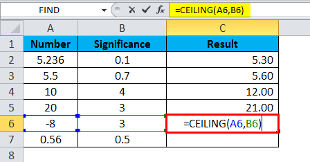
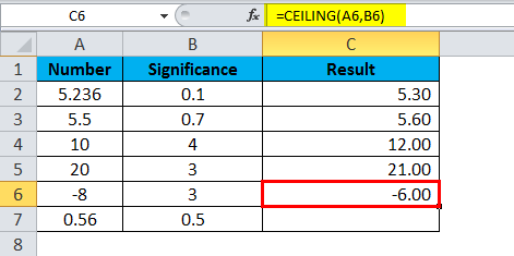
- CEILING also works for negative numbers too. In the fifth formula, the number is negative (-8), and the significance is positive (3). 3*3 = 9, which is nearest to 8. The Formula used is =CEILING(A6,B6)
Since it is a negative number, the formula returns the lower value, i.e. 3*2=6, and the supplied number is negative; the result also will be negative only (-6).
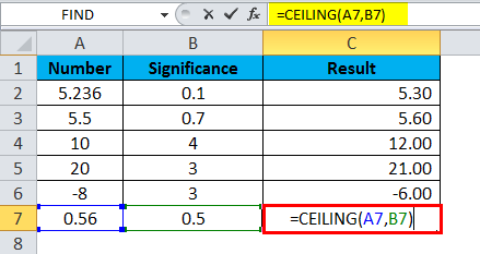
- Final formula is 0.5*2 = 1 that is round up of 0.56. 0.5*1 = 0.5 only this is lower than the original value of 0.56. Formula used is =CEILING(A7,B7)
The next highest value is 1.
Example 2
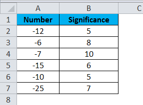
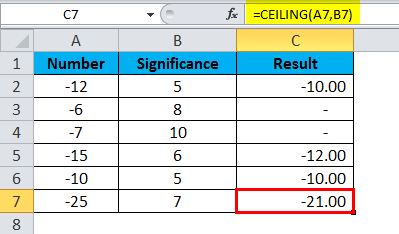
In the first example, we have seen positive numbers with positive significance. In this example, I will explain the scenarios of negative numbers with positive significance.
Negative numbers always round down the values, unlike positive numbers, which always round up the values.
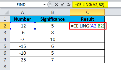
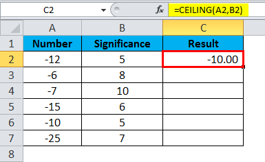
- In the first formula, the number is -12, and the significance is 5. Formula used is =CEILING(A2,B2)
Significance multiple is 5*2 = -10 which is nearest to -12 unlike 5*3 =-15.
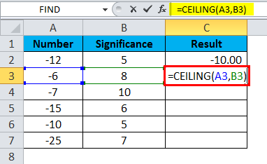
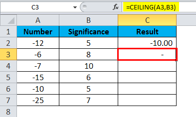
- The second formula returns 0; the reason behind this is the given number is -6, but we are multiplying values is 8, which always returns the value of more than 6. The formula used is =CEILING(A3,B3).
Therefore, the formula returns nothing.
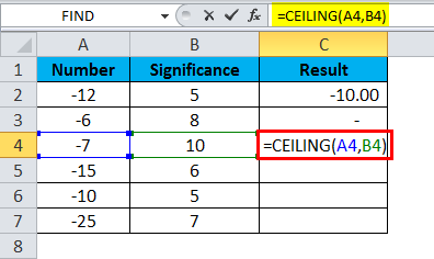
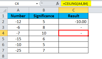
- Third, one is also the same as the second one. The significant number is more than the given number. Formula used is = CEILING(A4,B4).
The result will be zero.
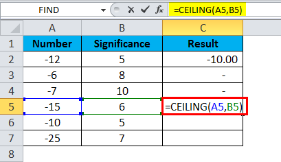
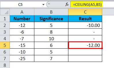
- In the fourth formula, a number is -15, and significance is 6. A formula used is =CEILING(A5,B5).
Significance multiple is 6*2 = -12 which is nearest to -15 unlike 6*3 =-18.
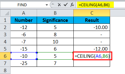
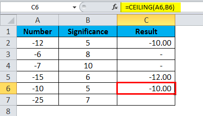
- In the fifth formula, a number is -10, and significance is 5. The formula used is =CEILING(6,B6).
The significance multiple is 5*2 = -10, which is equal to the given number.
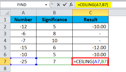
- In the sixth formula, the number is -25, and the significance is 7. The formula used is =CEILING(A7,B7).
Significance multiple is 3*3 = -21 which is nearest to -25 unlike 7*4 =-28.
Things to Remember
- In this function, the number always gets larger, i.e., round up always based on the multiple of significance number.
- The number should not be less than the significance numbers; otherwise, the result would always be zero.
- This formula does not accept values other than numeric values. If anyone of the supplied argument is non-numeric, then the result will be #VALUE!
- If the number is positive and the significant number is negative, we will get the error as #NUM! Therefore, if the significant number is negative, then the number also should be negative.
Recommended Articles
This has been a guide to the CEILING Function. Here we discuss the CEILING Formula and how to use the CEILING function along with a practical example and downloadable excel templates. You may also look at these useful functions in excel –

