CHAR Function in Excel (Table of Contents)
CHAR Function in Excel
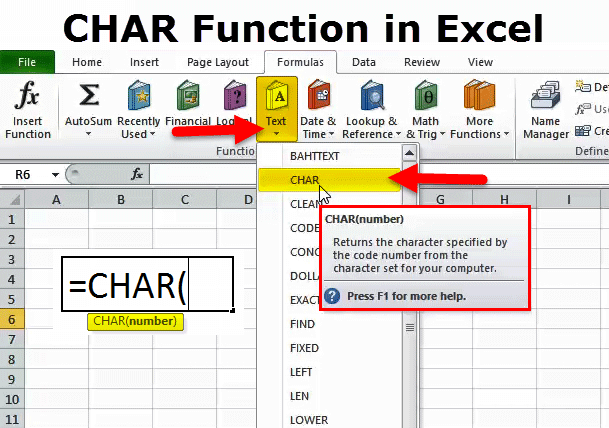
CHAR means CHARACTER. In Excel CHAR, the function is a TEXT formula that returns the character specified by numbers 1 to 255. Microsoft builds these characters based on the numbers that we supply. It is very useful to insert characters into our strings while writing something. These characters ordinarily cannot type from our normal keyboard. Instead, we need to use the CHAR function.
CHAR Formula in Excel:
The CHAR Formula in Excel is as follows.

The Formula of the CHAR function involves only one argument, i.e., the number
Number: It is the integer number ranging from 1 to 255.
This argument can be given cell reference and direct supply to the argument. Since we only need to supply numbers as an argument, we need not specify the number and double quotes.
How to Use CHAR Function in Excel?
This CHAR is very simple and easy to use. Let us now see how to use the CHAR Function in Excel with the help of some examples.
Example #1
Firstly, we need to look into which number specifies which character. The below list tells the associated character for each number.
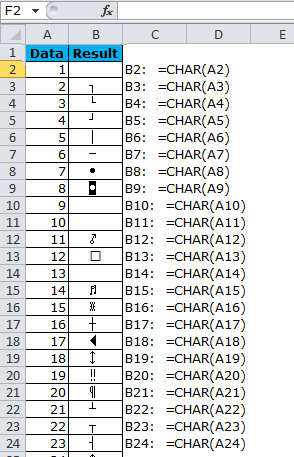
CHAR number 1 unleashes nothing, i.e., empty cell but only for the outset. There is always a character in it. You can use the LEN formula to check.

Example #2
Assume you are working in a college as an assistant. You have a list of all the students and must post the attendance report to their respective homes. You have addressed three different columns, and you need to merge those 3 into 1 column and insert line breakers after every column.
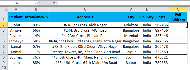
In column G, you must combine the full address by giving a line breaker after each address. We can insert the line breaker by using the CHAR function. Important to know which number to use to insert a line breaker. Number 10 we need to use to insert the line breaker after each address column.

Initially, our data looks like this. One tuning we need to do here. The tuning is we need to wrap the text to see the difference.
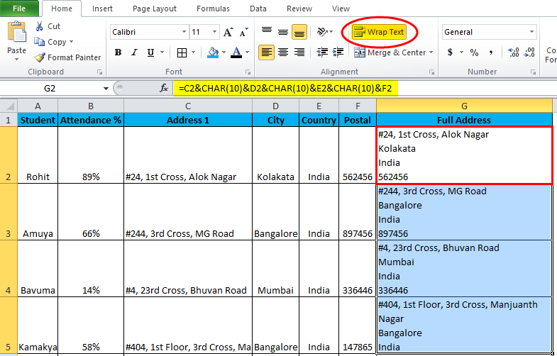
Now, see how your address column looks.
Example #3
We can insert alphabets by using the CHAR function. Below are the lists of numbers to insert in the alphabet.
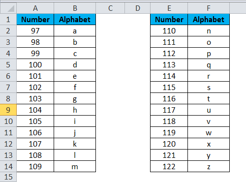
Apply these codes in Excel to see the magic.
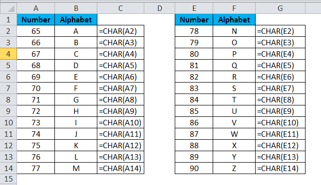
Now we have inserted UPPER case alphabets. We need to use the codes below to insert the LOWER case alphabets.
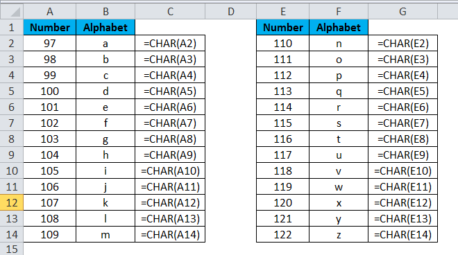
Example #4
We can insert those CHARACTERS by using the keyboard too. Below is the list of those keys.
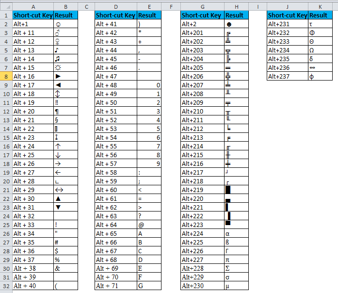
Example #5
Assume you downloaded the data below from the web and need to remove all those line breakers and special characters from this.

We can use the SUBSTITUTE function to remove those special characters and line breakers.
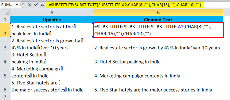
We have used a three-nested SUBSTITUTE function to remove special characters and line breakers.
Things to Remember
- CODE function can return the number if you give the special character as a reference. For example, =CODE (“A”) will return 65 as the answer.
- The first 32 are non-printable characters that can be removed using an Excel CLEAN function.
- We can insert the characters using ALT + numbers instead of the CHAR formula.
- If the supplied number is not triggered, we will get #VALUE! Error, i.e., numbers more than 255.
- We will get the same error if the supplied number is not in the numeric format.
Recommended Articles
This has been a guide to CHAR Function. Here we discuss the CHAR Formula, how to use CHAR Function in Excel, and Excel examples and downloadable Excel templates. You may also look at these useful functions in Excel –

