Updated August 11, 2023
Checkmark in Excel
A checkmark in Excel is a marking type used as a character in a cell. This becomes applicable only if we have selected the Wingdings2 fonts in Excel, mainly used for creating the marks. If we want to create a Checkmark into a cell, we need to type Shift + P or directly use capital P, which will return Checkmark. Even if we use the correct alphabet or character under Wingdings2 fonts, but the font size (Upper or Lower Case) needs to be properly used, we will get a different mark.
How to Insert Checkmark in Excel?
Let’s see how to insert a checkmark or tick mark in Excel.
A tick mark can be inserted into a cell to convey the result of “yes” as an answer to some questions, or the option “yes” applies here. There are two types of checkmarks in Excel.
- Interactive check box – Conveys a message to the next level.
- Tick symbol – This is a Special symbol.
Checkmark in Excel – Example #1
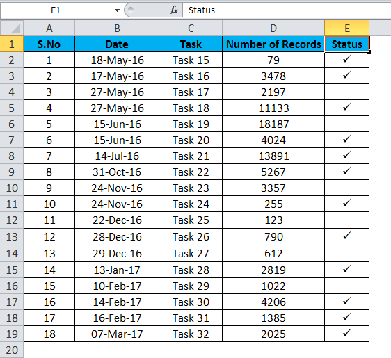
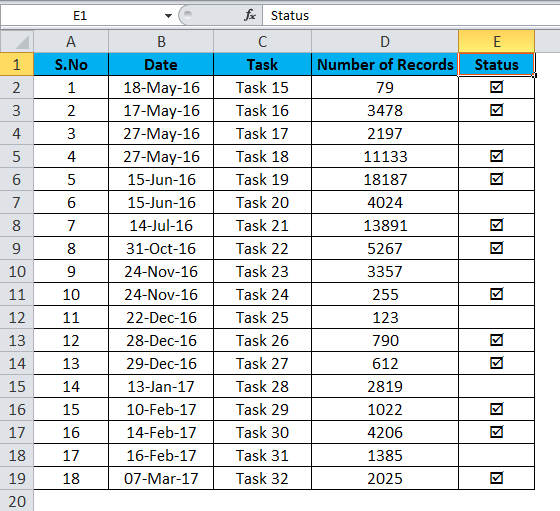
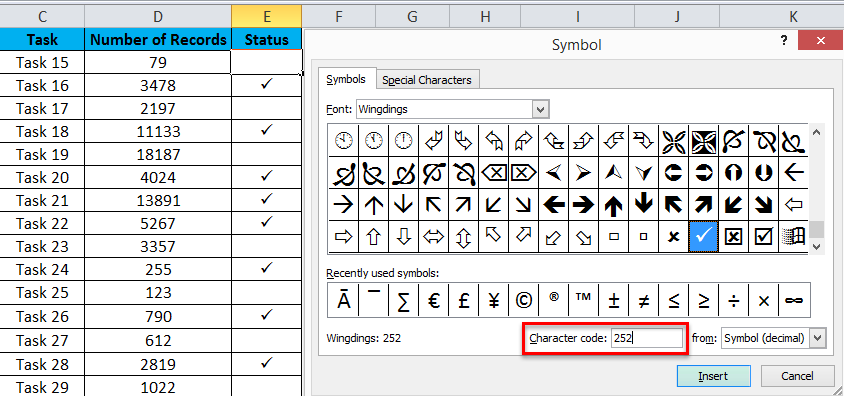
The sheet represents the status of which all the tasks are completed. The complete details are mentioned in the sheet, and a tick mark is given in the status column to mention the completed tasks. When the sheets contain complex data, it is easy to use tick marks instead of using any other comments.
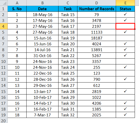
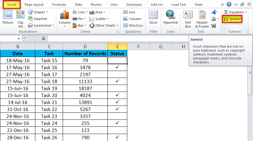
- Select the cell in the status column where you want to insert the tick mark.
- Go to the Insert menu and click on the symbols option. You will get the list of symbols in the dialog window.
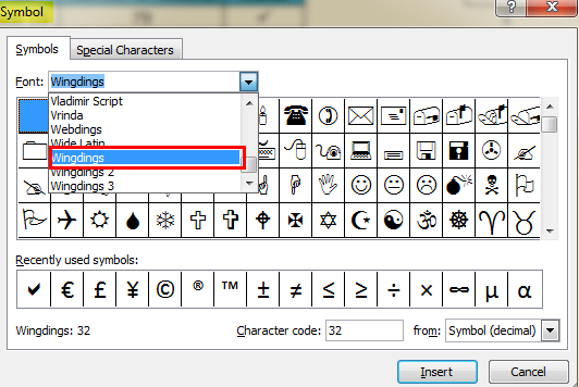
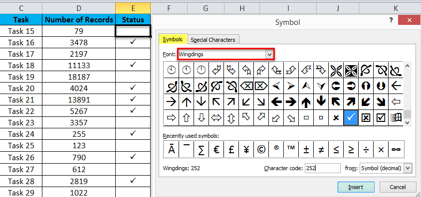
- Use the drop-down arrow from the symbol dialog window to select the font Wingdings.
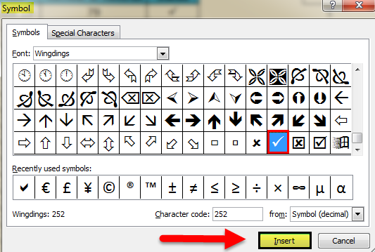
- With the dialog window, you can see different symbols. Select the tick mark and click the insert button to insert the symbol to the selected cell.
- Press the cancel button to hide the dialog window.
Checkmark in Excel – Example #2
Instead of a tick mark, we can use a tick box or checkbox to represent an option selected. This checkmark box can be used to show a Yes; this applies. Along with this, a cross mark is also used to indicate some incorrectness. Here the task which is completed is indicated by the tick box.
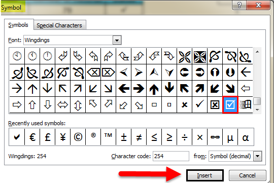
- Select the cell in the status column where you want to insert the checkbox. Go to the Insert menu and click on the symbols option. You will get the list of symbols in the dialog window. (As shown in the above steps)
- From the Symbol dialog window, use the drop-down arrow to select the font “Wingdings” (As shown in the above steps)
- With the dialog window, you can see different symbols. Select the checkmark symbol and click on the insert button to insert the symbol into the selected cell.
- Press the cancel button to hide the dialog window.
How to Use Tickmark in an Excel Sheet?
The simple way is to insert the tick mark symbol from the Symbols option.
- Select the particular cell where you want to insert the tick mark symbol.
- Go to the menu bar and select the insert option.
- From the Insert menu, go to the symbol option.
- From the Symbol dialog window, use the drop-down arrow to select the font “Wingdings.”
- With the dialog window, you can see different symbols. Select the tick mark and click the insert button to insert the symbol to the selected cell.
- Press the cancel button to hide the dialog window.
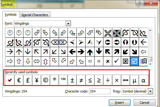
The same is shown in the figure where you can see the tick mark is being selected, and the same will be added to the “Recently Used Symbols” list.
How to Insert a Tick Mark using CHAR Function?
It is possible to insert the tick mark in Excel or checkbox using the char function, a built-in function in Excel. This is a simple way for those who commonly use formulas more in Excel.
While selecting the symbol in the dialog window, Excel generates a character code for every symbol.
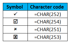
For example, the Character code for the tick mark is 252.
Use the formula =CHAR (252) to get the tick mark in the selected cell. Make sure that the font of the cell should be Wingdings.
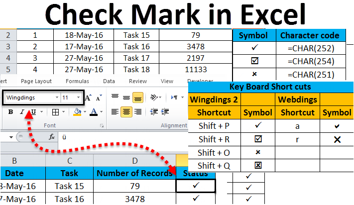
Use the below symbol code for inserting different symbols using the CHAR function.
How to insert a tick mark in Excel using keyboard shortcuts?
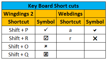
The symbols can be inserted in Excel using some keyboard shortcuts. It is commonly a combination of the shift key and an alphabet. Before applying the shortcuts, the cells should apply the “Windings 2” or “Webdings” font to get the below-given results.
This is also a simple method to insert the tick mark symbol in the cell where you want. Once you apply any of the mentioned fonts, press the shift key along with the alphabet P. You can see the tick mark appearing on the selected cell.
How to Insert a Checkmark in Excel with AutoCorrect?
This is another option on how to insert check marks in Excel. When you want to use this symbol regularly, this will be the easy way to insert the checkbox.
- Insert the tick mark symbol from symbols followed by inserting the menu
- Select the particular cell and copy the symbol from the formula bar
- Select the” ü” symbol and press “Ctrl + C” to copy it.
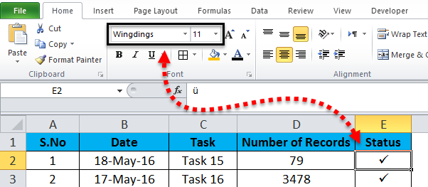
- Note the font type that is being selected; this will be needed while you are auto-inserting the tick mark.
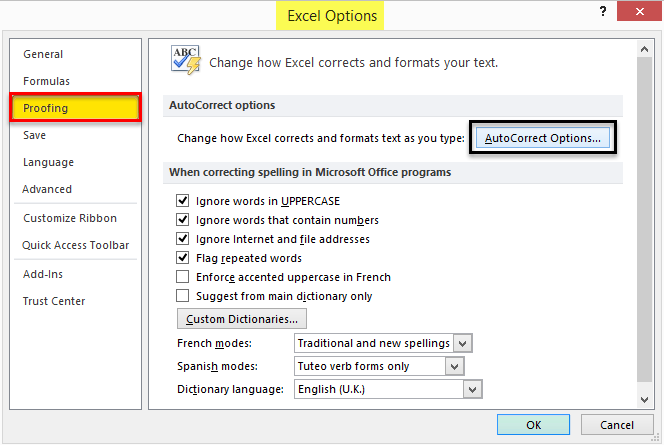
- Go to the File menu, then select options.
- Select “proofing “from the dialog window; also select the Autocorrect Options.
- Once you go through the Autocorrect option, you will get another dialog box.
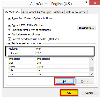
- In the “Replace” box, type the word which you want to use instead of the tick mark.
- In the “With” box, paste the copied symbol ” ü” (Ctrl + V)
- Press on Add button, then click OK
By following the mentioned steps, the tick mark symbol is auto-corrected. After completing this, go with the following steps when you want to put a tick mark on the Excel cell.
- Type the word you linked with the checkmark (Eg: tick mark) and enter.
- The symbol” ü” will appear in the cell. To change it into a tick mark, apply the proper font (i.e., Wingdings) to the cell.
The benefit of using this method is that you can associate the word you want with a particular symbol and remember it easily. Once you configure the Autocorrect option, you can add the symbol anytime by typing the associated word.
Things to Remember about the Checkmark in Excel
- When selecting from the insert symbol options, the symbol font should be in “Wingdings” in the dialog window.
- While using the character function, ensure the selected cells should be in “Wingdings” font to get the expected result.
- Use the Autocorrect method if you regularly use the same type of symbols.
- To find the character code for the symbol, select the symbol from the symbol window and check the corresponding character code in the box at the end of the symbol window.
Recommended Articles
This has been a guide on Checkmark in Excel. The easiest way to adjust a column is using the Excel Checkmark. Here we also discuss how to insert Checkmark in Excel, practical examples, and a downloadable Excel template. You can also go through our other suggested articles –
