Excel Choose Formula (Table of Contents)
Introduction to CHOOSE Formula in Excel
MS Excel provides several VBA inbuilt functions; one of them is Choose Function, which is used to choose a value by position or index from the given list of values. The Index number can be a number between 1 to 254, and values also can be 1 to 254 values.
The syntax of Choose Function: Choose()
It will return a value. There are two parameters or arguments required in the Choose Function- Index number and values.
How to Use CHOOSE Formula in Excel?
CHOOSE Formula in Excel is very simple and easy to use. Let us now see how to use the CHOOSE Formula in Excel with the help of some examples. These examples will surely help you with a clear understanding of the function.
Excel CHOOSE Formula – Example #1
Let’s assume there are five colors ‘Red’, ’Blue’, ’Black’, ’Pink’ and ‘Green’.
Now, if a user wants to choose a color based on its position. So, how a user will be able to choose a color based on its position.
As the user wants to choose a color based on its position, where he needs to use the choose function. so write the below formula in cell B1.
Now it will ask for the index number and values from where the user wants to choose a value. Now let’s assume a user wants to choose the 3rd value so that the index number will be 3. It will ask for values, so the user has five colors from where he wants to choose the 3rd value.
Click on the Enter button.
Summary of Example 1: As the user wants to choose the 3rd color from the given five colors ‘Red’, ’Blue’, ’Black’, ’Pink’ and ‘Green’. There is ‘Black’ in the 3rd position in the given order.
Same coming by the choose function. A user can change the value of the index number between 1 to 5. The result will come as per the index number is given in the function.
Excel CHOOSE Formula – Example #2
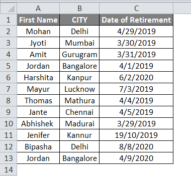
A user has staff details like the First Name, CITY, and Date of Retirement of their employee. Now the user wants to choose their city from the table.
So, how a user will be able to choose a city based on its position in the table.
Open MS Excel, go to sheet1, where the user wants to choose a city based on its position.
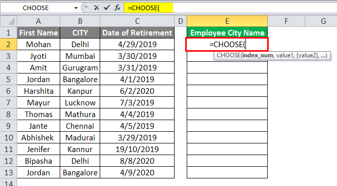
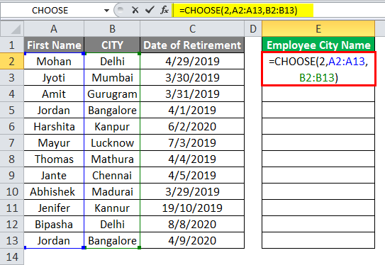
As the user wants to choose an employee city name based on its position in the table, where he needs to use the choose function. So, write the below formula in cell E2-
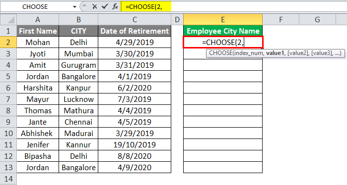
It will then ask for the index number and values from where the user wants to choose a value as the user wants to choose the city name for each employee available in the 2nd column of the table. So, the index number will be 2.
Now it will ask for values, so as a user, have some staff where everyone belongs to some city. Now he needs to select the range of name and city.
‘OR’
Just select the city range; that is also fine. This case index number will be 1 because there is only one value range selected: the city.
=CHOOSE (1, B4: B15)
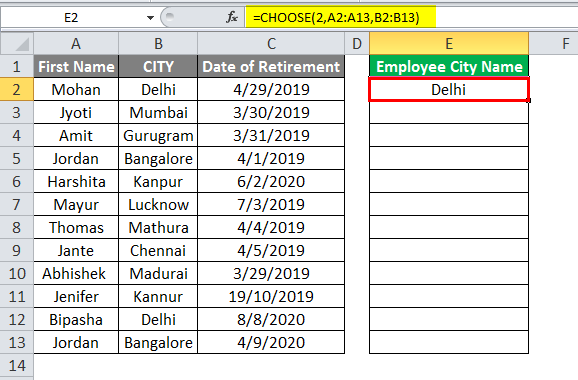
For now, we are taking the first name of the employee and city name in the value. Now click on the enter button.
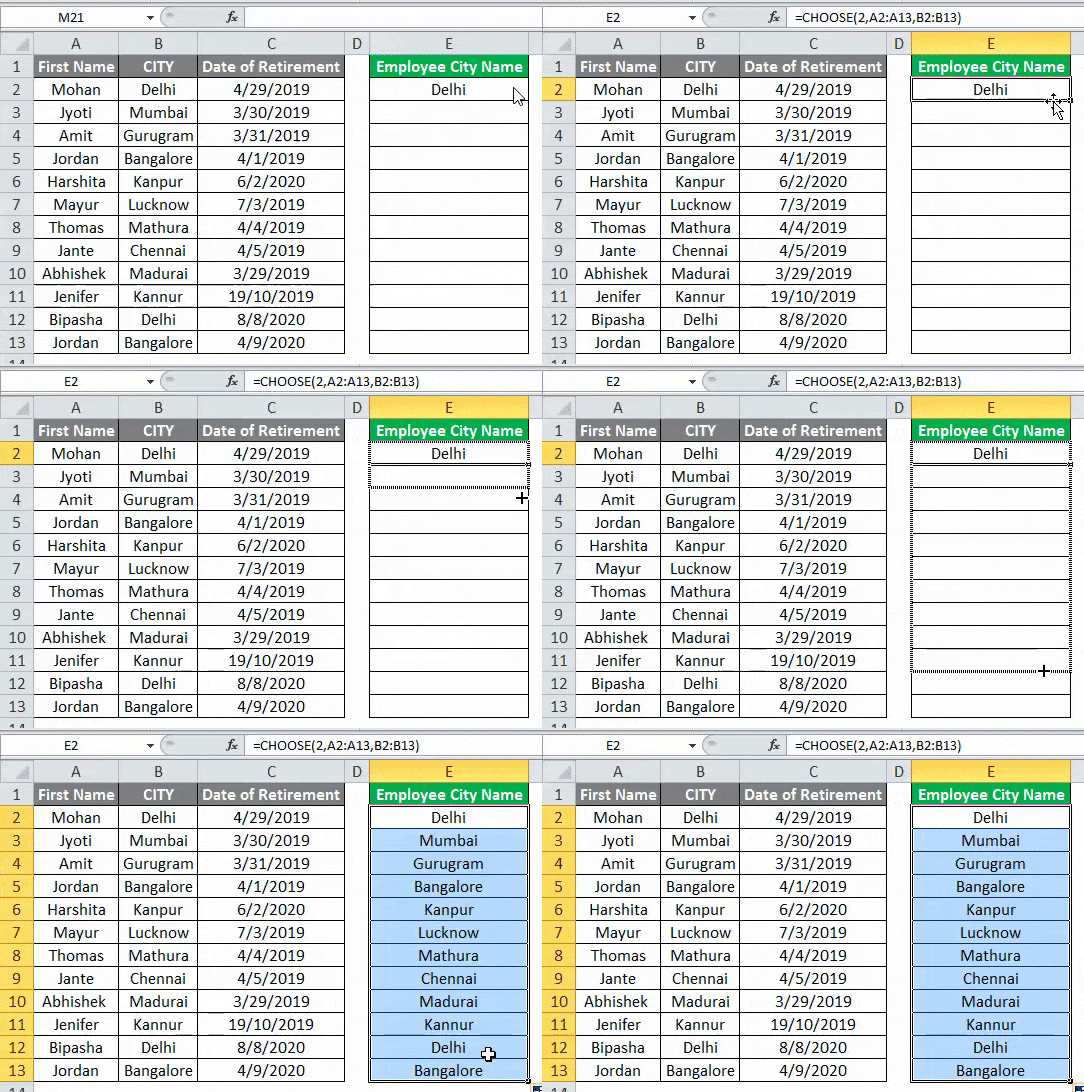
Just apply the same formula to the cell E5 to E15 by dragging the E4 formula.
Summary of Example 2: As the user wants to choose his staff’s city name from the given staff data table. In a similar way, a user can choose the first name, city, or date of retirement of his/her employee.
Same coming by the choose function. A user can change the value of the index number between 1 to 3. The result will come as per the index number is given in the function.
Excel CHOOSE Formula – Example #3
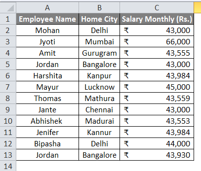
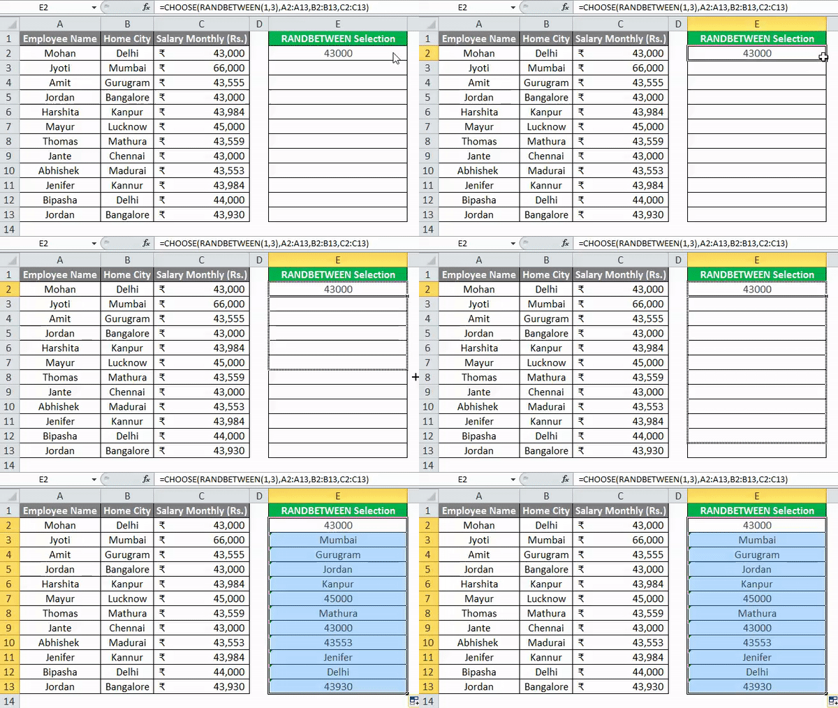
A user has staff details like Employee Name, Home city, and Salary Monthly (Rs.) of their employees.
Now the user wants to choose their random data from the employee details table so, how a user will be able to choose random data based on its random position in the table.
Open MS Excel, go to sheet2, where the user wants to choose random data based on its position.
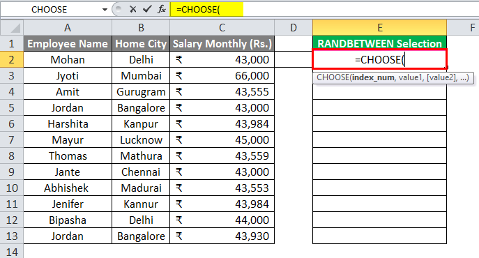
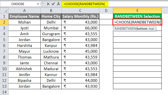
As the user wants to choose employee random data based on its position in the table, where he needs to use the choose function with the RANDBETWEEN excel function. So, write the below formula in cell E2-
Now it will ask for the index number and values from where the user wants to choose a value.
As the user wants to choose random employee data that is available in the employee table. So, he needs to use the RANDBETWEEN function.
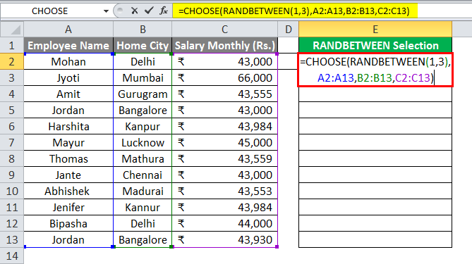
Now It will ask for values. So, just select all data range and give the RANDBETWEEN range 1 to 3.
=CHOOSE (RANDBETWEEN (1,3),A2:A13,B2:B13,C2:C13)
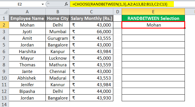
Now click on the enter button.
Just apply the same formula to the cell E3 to E13 by dragging the E2 formula.
Summary of Example 3: As the user wants to choose the random data of staff from the given staff data table. As we can see from the result, random data is coming from the staff details.
There is Employee name, Home city or Salary appearing in column E as random. It will change every time when the user changes any data in the table.
Things to Remember
- The Index number can be a number between 1 to 254, and values also can be 1 to 254 values.
- Index number always will be a number. It cannot exceed the total number of values given in the choose function. Otherwise, it will give an error #VALUE.
- If the Index number is a fraction, then it will automatically delete the fraction part to the nearest integer number.
Recommended Articles
This has been a guide to CHOOSE Formula in Excel. Here we discuss How to use CHOOSE Formula in Excel along with practical examples and a downloadable excel template. You can also go through our other suggested articles –
