Updated August 16, 2023
Circular Reference in Excel
Circular Reference in Excel is a kind of alert message we can see when selecting the values as a Circle in any formula. Rectifying circular references is important; otherwise, our applied formula will give us the incorrect value.
For example, if we sum the value of 5 cells into the 6th cell and mistakenly consider the range of 6 cells, including the cell where we will see the output, then although we would get the output, it will be an incorrect value. We can enable or disable Circular reference from Excel Options’ Formulas section.
How to Use Circular Reference in Excel?
Using It is very simple and easy. Let’s understand the situation of the Circular Reference error with some examples.
Example #1
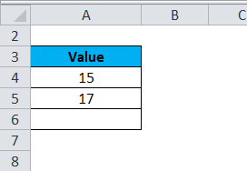
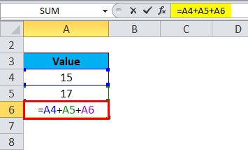
- As we can see, Cell A4 and A5 have some value, and in Cell A6, we have to add those values, including the value in Cell A6 itself.
- So we enter the formula like the below screenshot.
- When we hit the enter key, it will display an error message, as shown below.
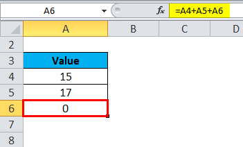
- If you click OK or close the window by clicking the cross button, Excel will take it as a Zero value or the last calculated value in the cell.
- If you click on Help, you can get more information.
- We have clicked OK, which will display 0 in cell A6. ( Refer to the below screenshot )
You might be surprised that Excel will sometimes complete the formula with the last calculation having a Circular reference condition without displaying an error message and returning the value in the cell.
In some conditions, we might require to create a circular reference while calculating. Let’s take an example to create that scenario where circular reference must be included.
Example #2
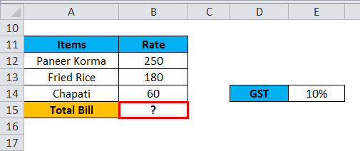
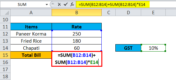
Suppose you go to a restaurant and have lunch. You get the bill which you have to pay before leaving. The GST ( Goods and Service Tax ) on total expenses is 10%, so we must calculate the total bill.
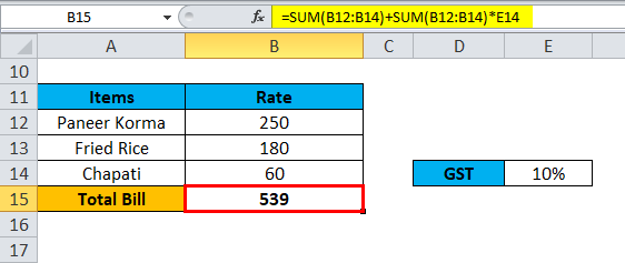
Here, we will apply the formula in the below screenshot.
Here we will sum up all the Item prices and calculate the 10% on that amount. Then will add this tax amount to the total item’s price. It will give you the total expenses.
But here, Circular reference is a part of the formula; it won’t calculate the total bill. So in this situation, we need to make some changes in Excel settings for further calculation.
This scenario will display an error message, as shown in Example 1 ( Figure 3 ).
Find Circular Reference in Excel
Follow the below steps :
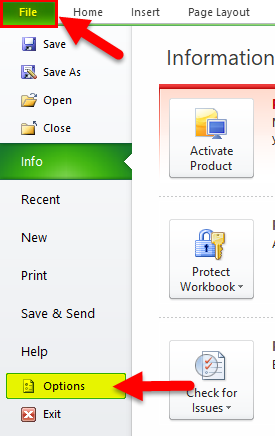
- Go to the FILE tab.
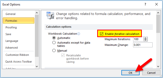
- Click on Options in the left pane window. Then, refer to the below screenshot.
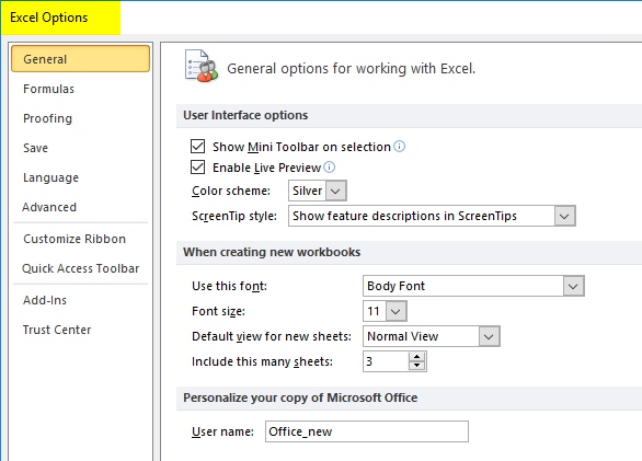
- It will open a dialog box for Excel options.
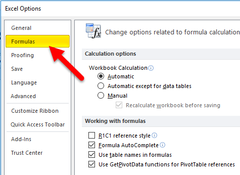
- Click on the Formulas tab.
- Tick on the “Enable iterative calculation” checkbox, as shown in the screenshot below.
- Click on OK.
- It will calculate the Total Bill in Cell B15. Refer to the below screenshot.
By enabling this Iterative calculation option, it will repeat the re-calculation until a specific numeric condition is met.
There are two ways to turn on this option.
We can see two options available under the Enable iterative calculation section, as shown in the screenshot below.
- Maximum Iterations: As we can see here, the default value is 100. This means Excel will repeat the calculations 100 times and try to solve this.
- Maximum Change: Excel will try to repeat the calculation 100 times and stops when it finds the difference is not more than 0.001 between iterations.
Things to Remember
- We should avoid Circular reference, the reason being, it leaves an impact on the performance and displays a warning message every time at the time of opening the workbook.
- It can also be the reason for other issues that are not immediately visible.
Recommended Articles
This has been a guide to Circular Reference in Excel. Here we discuss finding and using a circular reference in Excel, practical examples, and a downloadable Excel template. You can also go through our other suggested articles –
