Updated August 16, 2023
Columns to Rows in Excel
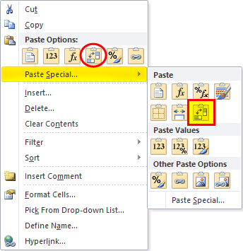
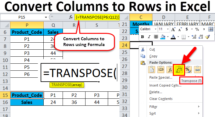
In Excel, select the column you want to switch and copy the selected cells or columns to convert any Columns to Rows. Go to the cell where you want to paste the data. Then, select the Transpose option from the Paste option under the Home menu tab. This will convert the selected Columns into Rows. You can also use the shortcut keys Alt + H + V + T, which will directly take us to the TRANSPOSE function.
Paste Special Option.
The shortcut key for paste special:
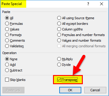
Once you have copied the range of cells that need transposed, click on Alt + E + S in a cell where you want to paste a special dialog box popup window with the transpose option.
How to Convert Columns to Rows in Excel using Transpose?
Converting data from column to row in Excel is very simple and easy. Let’s understand the working of converting columns to rows by using some examples.
Example #1
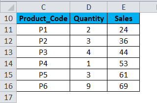
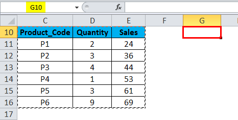
The below-mentioned Pharma sales table contains the medicine product code in column C (C10 to C16), quantity sold in column D (D10 to D16) & total sales value in column E (E10 to E16).
Here we need to convert its orientation from columns to rows with the help of a special paste option in Excel.
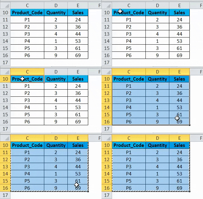
- Select the whole table range in a spreadsheet, i.e., all the cells with the dataset.
- Copy the selected cells by pressing Ctrl + C.
- Select the cell where you want to paste this data set, i.e., G10.
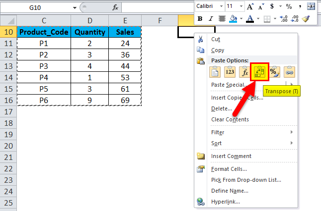
- When you enable right-click on the mouse, the paste option appears. You must then select the 4th option, i.e., Transpose (As mentioned in the below screenshot)
- On selecting the transpose option, your dataset gets copied in that cell range, starting from cell G10 to M112.
- Apart from the above procedure, you can also use a shortcut key to convert columns to rows in Excel.
- Copy the selected cells by pressing Ctrl + C.
- Select the cell where you must copy this data set, i.e., G10.
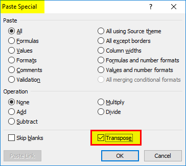
- Click on Alt + E + S, and paste a special dialog box popup window that appears, select or click on the box Transpose option, and it will result in or convert column data to rows data in Excel.
Copy data is called source data, and when this source data is copied to other ranges, i.e., pasted data, which is referred to as transposed data.
Example #2
Sometimes, when you have a huge number of columns, column data at the end is not visible and does not fit to screen. In this scenario, you can change its orientation from the current horizontal range to the vertical range with the help of the paste special option in Excel.
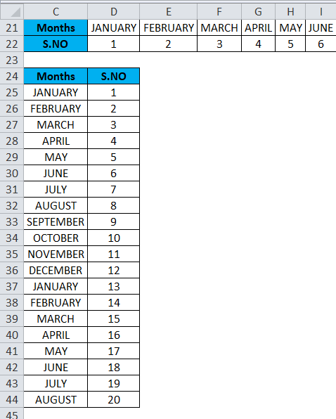
- The table contains months and their serial number (From columns C to W).
- Select the whole table range in a spreadsheet, i.e., all the cells with the dataset.
- Copy the selected cells by pressing Ctrl + C.
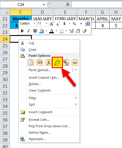
- Select the cell where you must copy this data set, i.e., C24.
- When you right-click on the mouse, the paste options appear, in that you have to select the 4th option, i.e., Transpose (Below mentioned screenshot)
- On selecting the transpose option, your dataset gets copied in that cell range starting from cell C24.
In the transposed data, all the data values are visible and clear compared to the source data.
Disadvantages of using the Paste special option:
- Sometimes copy-paste option creates duplicates.
- If you have used the Paste special option in Excel to convert columns to rows, the transposed cells (or arrays) are not linked to each other with source data, and it does not get updated when you try to change data values in the source data.
Example #3
The transpose function converts columns to rows and rows to columns in Excel.
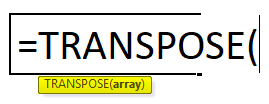
The syntax or formula for the Transpose function is:
- Array is a range of cells you need to convert or change their orientation.
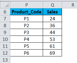
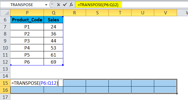
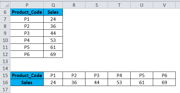
Check out the number of rows & columns in the source data you want to transpose. In the below example, the Pharma sales table contains the medicine product code in column P (P7 to P12) and sales data in column Q (Q7 to Q12).
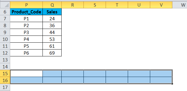
i.e., Initially, count the number of rows and columns in your original source data (7 rows & 2 columns), which is vertically positioned. Now select the same number of blank cells, but in the other direction (Horizontal), i.e. (2 rows & 7 columns)
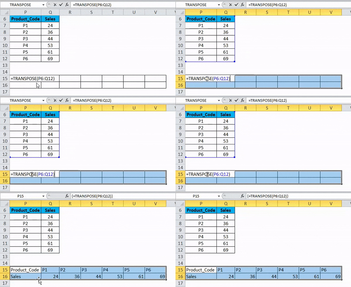
- Before entering the formula, select the empty cells, i.e., from P15 to V16.
- With the empty cells selected, Type the transpose formula in cell P15. i.e. = TRANSPOSE (P6:Q12).
- To apply the formula for the whole range, press Ctrl + Shift + Enter, converting it into an array formula.
Now you can check the dataset; columns are converted to rows with datasets.
Advantages of the TRANSPOSE function:
- The main benefit or advantage of using the TRANSPOSE function is that transposed data or the rotated table retains the connection with the source data. Whenever you change the source data, the transposed data also changes accordingly.
Things to Remember About Convert Columns to Rows in Excel
- Paste special option can also be used for other tasks, i.e., Add, Subtract, Multiply, and Divide between datasets.
- #VALUE error occurs while selecting the cells, i.e., If the number of columns and rows selected in transposed data is not equal to the rows and columns of the source data.
Recommended Articles
This has been a guide to Columns to Rows in Excel. We have discussed converting columns to rows in Excel using transpose, practical examples, and a downloadable Excel template. Transpose can help everyone to convert multiple Columns to Rows in Excel easily and quickly. You can also go through our other suggested articles –
