Updated August 9, 2023
Complex Formulas in Excel (Table of Contents)
- Introduction to Complex Formulas in Excel
- Choose Function Serve as Lookup Function
- VLOOKUP With CHOOSE
- IF With AND & OR Function
Introduction to Complex Formulas in Excel
Excel comes with many useful formulas; we have a category of Financial, Logical, Text, Date & Time, Lookup & References, and Math & Trig”. Each individual formulas are good enough for intermediate users where they face straight forward situations, but as you progress to the next level, your skill needs to take the elevation, so in that regard, applying more complex formulas in excel plays a vital role in solving complex situations. Keeping this in mind, this article, we will take you through some of the important and much-needed complex formulas. Read on.
Choose Function Serve as Lookup Function
Not many of you have used CHOOSE function, but this is very useful to serve as the lookup function as well.
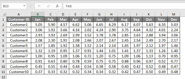
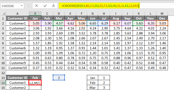
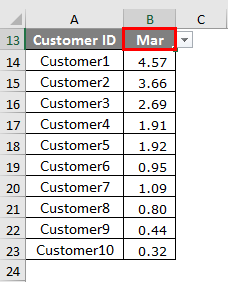
We have data of customers on a monthly basis under this table; we have each customer table. In this table, in cell B13, I have created the drop-down list of the month so that when this drop-down changes, we should get the total of the selected month.
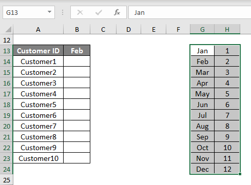
Create one table like the one below.
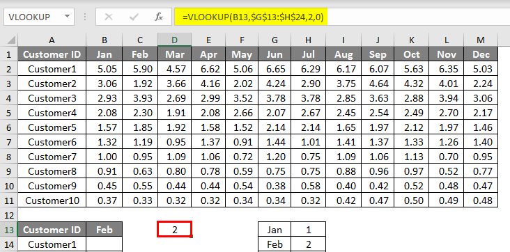
Apply VLOOKUP to cell D13.
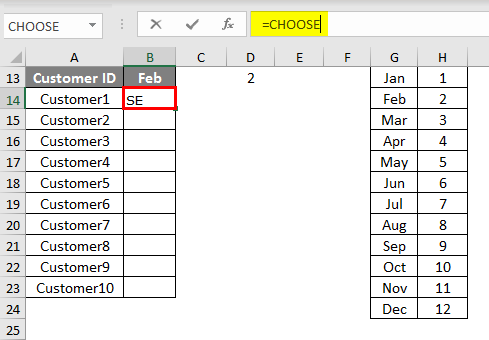
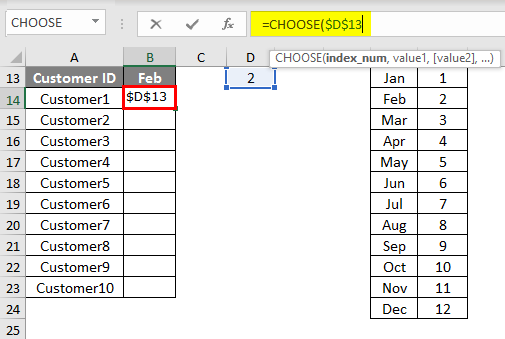
Now open CHOOSE function in cell B14.
Select the INDEX Number as a VLOOKUP cell and make it an absolute reference.
Now select for each argument each month sales numbers.
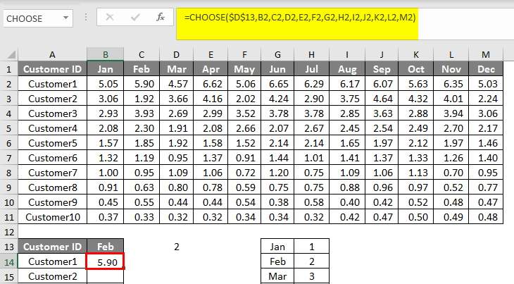
Close the bracket and hit the enter key.
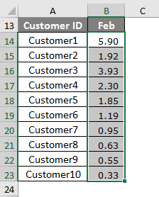
Now copy and paste the formula to the below cells as well.
Now CHOOSE formula will show the numbers of the selected month.
VLOOKUP With CHOOSE Function
We have seen tradition VLOOKUP, but we can combine it with CHOOSE function as well. For example, look at the below data.
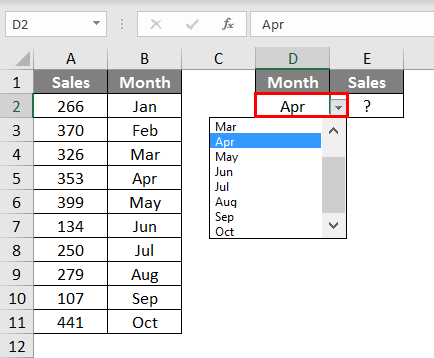
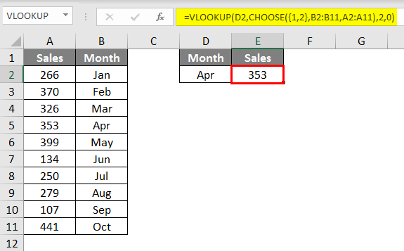
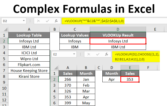
In cells A1 to B11, we have a sales table, and in cell D2, I have created the drop-down list of months, and in cell E2, we need to apply VLOOKUP and get the selected month sales value. But the problem to apply VLOOKUP is a data structure, where the lookup value is to the right of the result column, so VLOOKUP cannot fetch the data from right to left; in this case, we can use CHOOSE function.
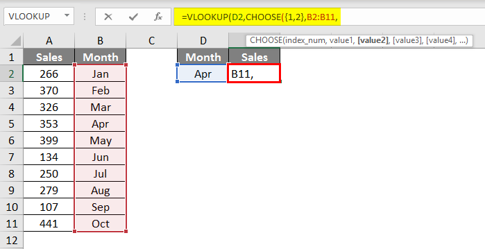
In order to select the table array, we need to open the CHOOSE function here.
In the INDEX Number argument in flower, brackets enter 1 & 2. Now select the first range as the Month column.
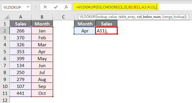
Select the Sales column as the second range.
Mention column index number as 2 and range lookup as 0.
So we got the result for the month of Apr from the table. So, whenever you don’t have an accurate data structure, we can select, CHOOSE function.
IF With AND & OR Function
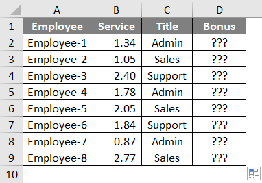
Logical functions are full of logic to calculate the stuff. Take a look at the below example data.
From the above table, we need to calculate the bonus based on the below conditions.
- If the Service is more than 1.5 years and if the department is either Sales or Support, then Bonus is 1000.
- If anything else, then Bonus is 3000.
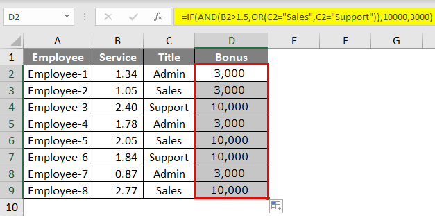
To calculate the bonus, we need to apply IF, AND, & OR together. Open IF condition in cell D2.
We need to test multiple conditions, open AND function.
Now the next logical is either Sale or Support so, for this open OR condition.
Test whether the title is Sales or Support.
So, if all the supplied conditions are TRUE, then the bonus should be 10000.
If the supplied logical tests are FALSE, then the bonus is 3000.
Close the bracket and hit Enter key; we should get the result.
Copy and paste the formula to the below cells.
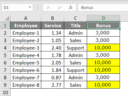
So, according to the condition, we got the result. If the service is >1.5 years and the title is either Sales or Support, we will get 10000 or else we will get 3000.
Complex Formula with Wildcard Characters
VLOOKUP requires an exact lookup value to be matched to fetch the data. This is the traditional slogan, but we can still fetch the data by using the particle lookup value. For example, if the lookup value is “VIVO” and in the main table, we can still match using wildcard characters if it is “VIVO Mobile”. We will see one of the examples now; below is the example data.
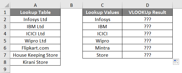
We have Lookup Table in column A. In column C, we have lookup values; these lookup values are not exactly the same as the lookup table values. So we will see how to apply VLOOKUP using wild cards.
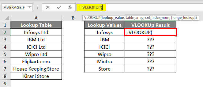
First, open the VLOOKUP function in cell D1.
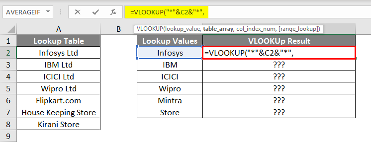
The first argument is the Lookup Value. One of the problems with the lookup value here is we don’t have an exact match, so we need to enclose this lookup value with an asterisk before and after the lookup value.
Here we have applied two asterisk characters, “*”&C2&”*”. Here asterisk indicates anything in between the wildcard should be matched and return the related result.
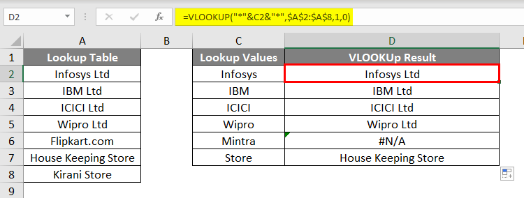
Even though we had just “Infosys”, the asterisk character matched the value in the lookup table and returned the exact result as “Infosys Ltd”.
Similarly, in cell D6, we got an error value as #VALUE! Because there is no word “Mintra” in the lookup table.
Recommended Articles
This is a guide to Complex Formulas in Excel. Here we discuss some of the important and much-needed complex formulas with examples and excel template. You can also go through our other suggested articles to learn more –
