Updated June 9, 2023

Excel Conditional Formatting for Blank Cells
Conditional Formatting for Blank Cells is the function in Excel that is used for creating inbuilt or customized formatting. From this, we can highlight the duplicate, color the cell as per different value ranges, etc. It also has a way to highlight blank cells.
How to Apply Conditional Formatting for Blank Cells?
Apply Conditional Formatting for Blank Cells is very simple and easy. Let’s understand how to apply it in Excel.
Example #1
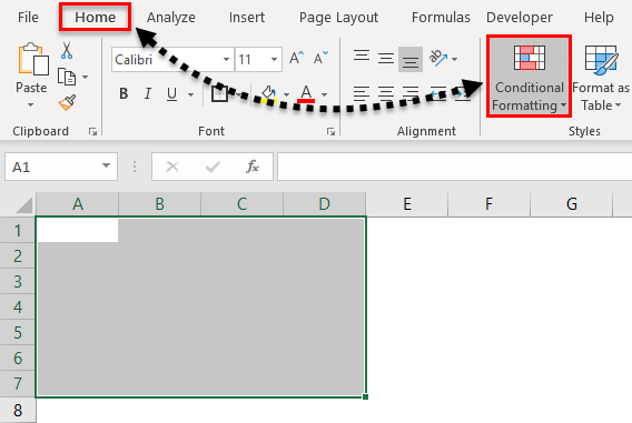
We will cover the small portion of Conditional Formatting, which Highlights the Blank Cells. For this, consider a blank sheet. This is the best way to see and apply conditional formatting for a blank sheet or some of the cells of a blank sheet. If we apply the conditional formatting to complete a blank sheet or some cells, we will see how the cell gets highlighted. For this, we have selected a small portion of the sheet covered with a thick border, as shown below.
- We will apply the conditional formatting in a defined region only. Go to the Home menu and select Conditional Formatting under the Styles section, as shown below.
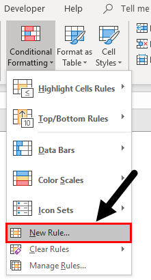
- Once we do that, we will get the drop-down list of Conditional Formatting. From that list, select New Rule.
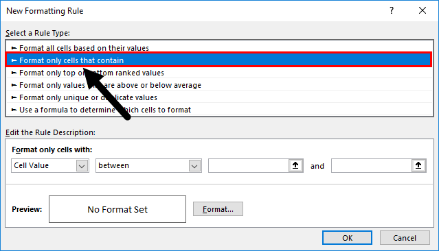
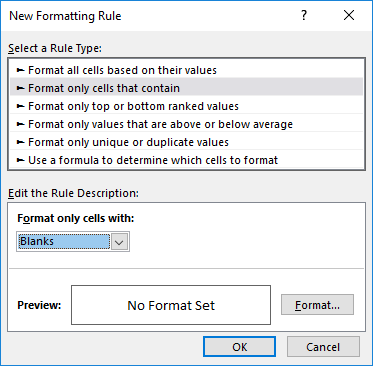
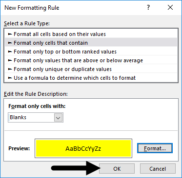
- There we have a different rule to apply conditional formatting. A window of the New Formatting Rule will open up. But for Blank cell, select the second option, Format only cells containing.
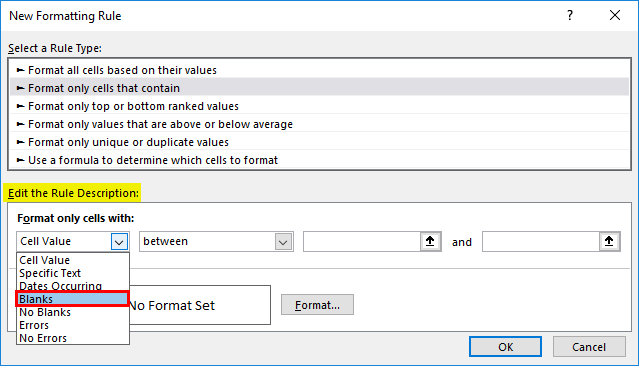
- And below, in Edit the Rule Description box, we have different criteria to define. Here, select Blanks as the cell value from the first box of the drop-down.
- Once we select the Blanks as cell value, all rest of the drop-down boxes will be eliminated from the condition. And we will get conditions related to Blank cells.
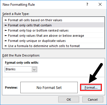
- Now, Click on the Format option from the same window as highlighted in the screenshot below.
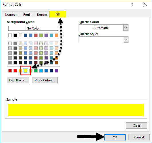
- The Format option will take us to the customize windows where we can change the text fonts and shape, define, or change the border or fill. We can also change the pattern as well. To highlight blank cells, go to the Fill tab and select any desired color as required. Once done, click on Ok, as shown below.
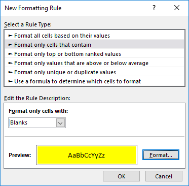
- After clicking on Ok, it will take us again back to the previous window, where we will get the preview of the selected color and condition as shown below.
- Here we got to apply conditions and rules as per our needs. If the selected condition suits and matches the requirement, click Ok or return to Format to update the conditions. Now click on Ok.
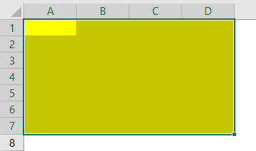
- After clicking Ok, we will get all the blank cells highlighted with Yellow color, as shown below.
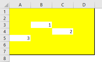
- Now to test whether the condition we selected is applied properly, go to any of those cells and type anything to see if the cell color changes to No Fill or White background. As we can see, the cells with any value are now changed to a No Fill cell, as shown below.
Example #2
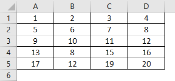
There is another way to apply conditional formatting to blank cells. And this method is quite easy to apply. For this, we have another set of data, as shown below.
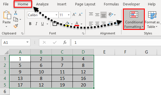
Now for applying Conditional Formatting, first select the data and follow the same path as shown in example-1.
- Go to the Home menu, under the Styles section, and select Conditional Formatting.
- Once we do that, we will get the drop-down list of all the available options under it. Now select the New Rule from the list.
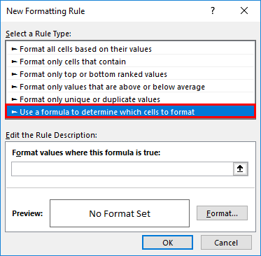
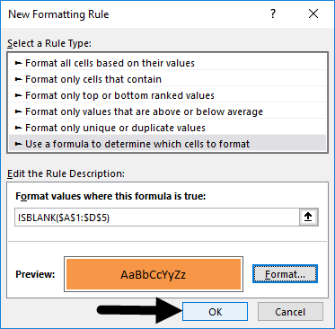
- Once we do that, we will get the New Formatting Rule box. There we have a different rule to apply conditional formatting. But here, we have to select the last option: “Use a formula to determine which cells to format”.
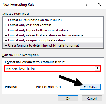
- Now in the Edit the Rule Description box, write the syntax of a function ISBLANK and select the complete range of data, and after that, click on the Format tab, as shown below.
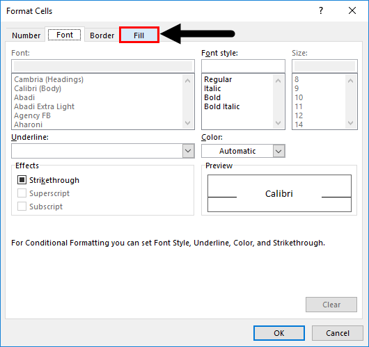
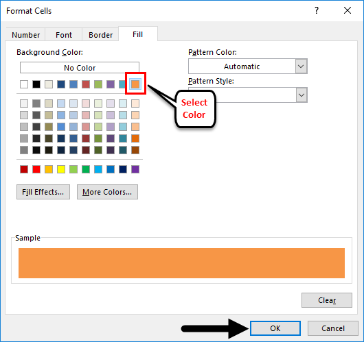
- Now a Format Cells window will open. Go to the Fill tab.
- And select the color of your choice to highlight the blank cells. Here we have selected the color as shown below. Click on OK to apply. Once done.
- After clicking on Ok, it will again take us back to the same previous window, where we will get the preview of the selected color and condition. Now click on Ok to apply.
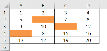
- To test the applied condition, delete any cell data and see the result. We have deleted some cell data for testing, and the color of those cells change from No Fill to Red Peach. Which shows our selected and applied conditions are working properly.
Pros
- It is very quick and easy to apply.
- We can select any range and type of data to highlight blank cells.
- This is quite useful when we are working on data validation work. By this, we can highlight the cell and attributes left blank.
Cons
- Applying conditional formatting to large data set such as complete sheet may make Excel work slow while filtering.
Things to Remember
- The selection of proper rules and formatting is very important. Once we select it, it will always check and look for the preview before applying the changes.
- Always use limited data to deal with and apply bigger conditional formatting to avoid Excel getting frozen.
Recommended Articles
This has been a guide to Conditional Formatting for Blank Cells. Here we discuss how to apply Conditional formatting for blank cells, practical examples, and a downloadable Excel template. You can also go through our other suggested articles –
