Updated May 3, 2023
DATEVALUE Function (Table of Contents)
DATEVALUE in Excel
The dateValue function in Excel converts the dates in text format into the standard Short Date format available in Excel. Suppose we feed “01 Jan 2020” as a text date; then the DateValue function will convert this into “01/01/2020”, which is purely a date format in Excel. For this, we need to supply the text date into the syntax of the DateValue function in double inverted commas. And also, if we do not mention the year while supplying the input, it will automatically consider the current year.
DATEVALUE Formula in Excel:
Below is the DATEVALUE Formula:
Arguments of DATEVALUE in Excel :
This DATEVALUE uses the below-mentioned arguments
date_text:- This argument represents text that represents a date in proper excel date format.
How to Open DATEVALUE Function in Excel?
Below are the steps to open the DATEVALUE Function in Excel.
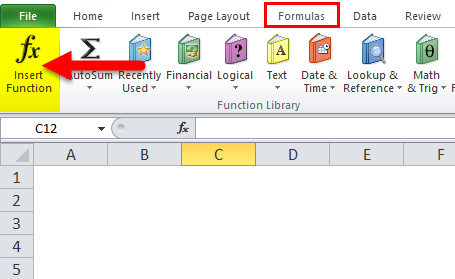
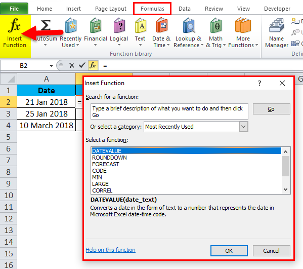
- Go to Formula Menu. Click Insert Function.
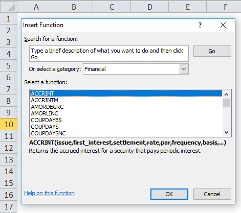
- A dialogue box appears as follows.
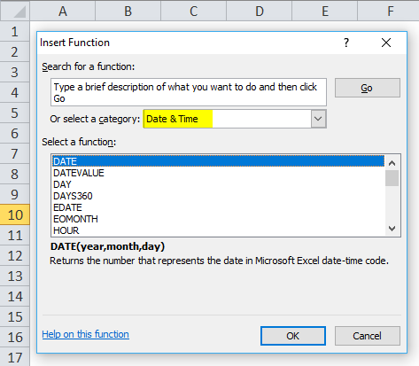
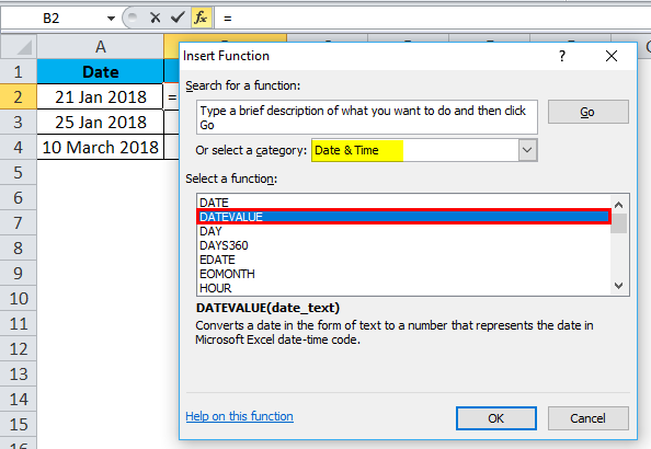
- Choose DATE/TIME Function
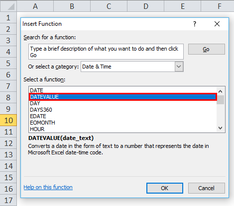
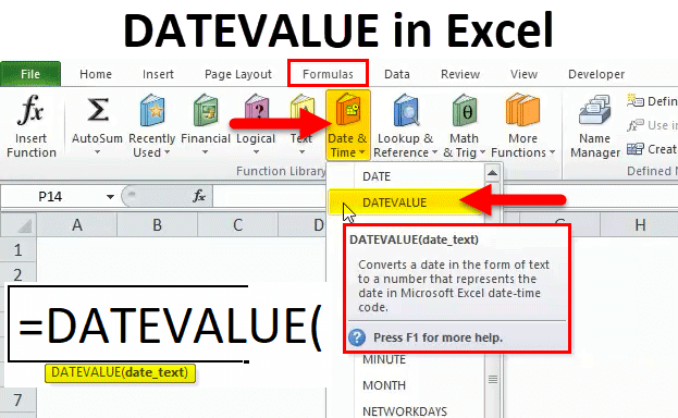
- Once you choose the DATE/TIME function, we will get a list of functions and then choose the DATEVALUE function.
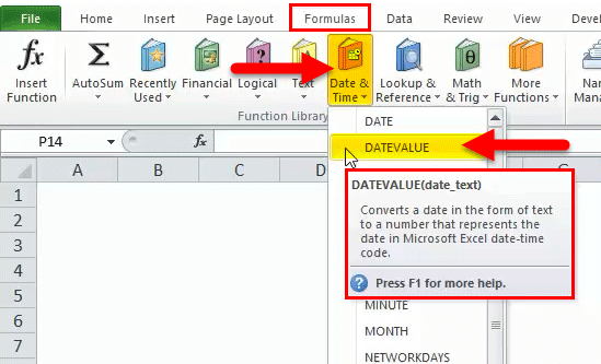
In the advanced version, we can find the shortcut in the formulas menu, like DATE and Time Function. Here we can select the category DATE/TIME function, and it will list a set of functions where we can find the DATEVALUE function in the list, shown in the screenshot below.
How to Use the DATEVALUE Function in Excel?
DATEVALUE Function is very simple to use. Let us now see how to use the DATEVALUE function in Excel with the help of some examples.
Example #1
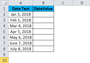
This example shows that we have two columns named Date Text and DateValue, Where Date Text only contains text with Month Day and Year.
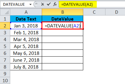
Now, let’s use the DATEVALUE function to convert the date text to the proper date format. Insert the function DATEVALUE by selecting the corresponding cells =DATEVALUE(A2)
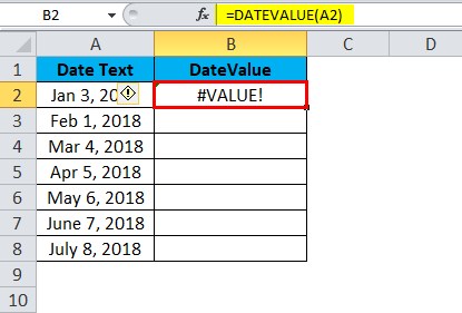
Once we hit the enter key, the following results will be displayed: DATEVALUE returns strings of serial numbers; to display in date format, we need to format the cells to date format.
Here in the above screenshot, we can notice that we got a #VALUE error; we can wonder why we got this error because there will be several reasons like the date text argument will be a value in date format or the date text argument will be a value in number format or date settings might be set to MM/DD/YYYY format. It should not be in DD/MM/YYYY format.
In order to overcome this error value, we need to format the cells to date format.
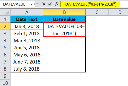
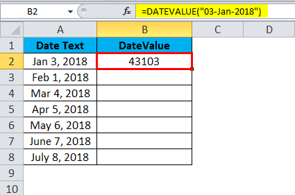
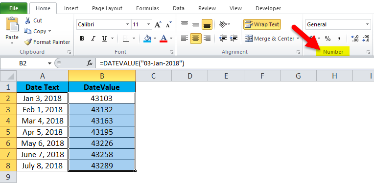
Another option where we can avoid this #VALUE error is can enter DATEVALUE by inserting the date within the quotation, i.e. =DATEVALUE (“03-Jan-2018”) as shown in the below screenshot.
The Result is:
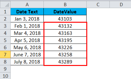
Similarly, We can Find other Value
Now Excel treats the above function as text (strings), and it can be changed to date format by formatting the cells as shown below.
We can format the cells by following the below steps;
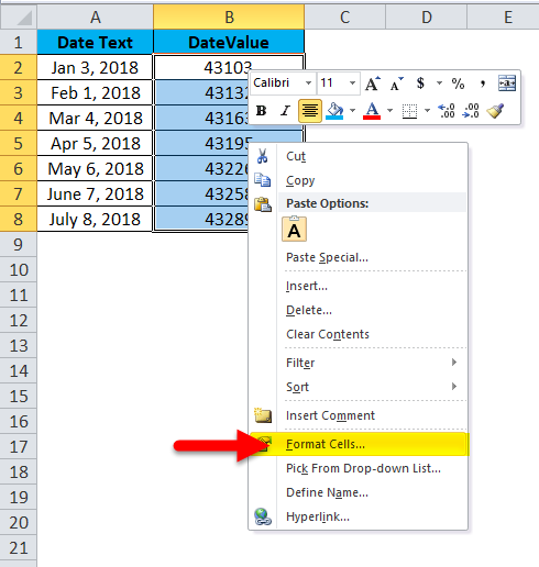
- First, select the cell
- Right-click on the cell. You will get option format cells, as shown in the below screenshot.
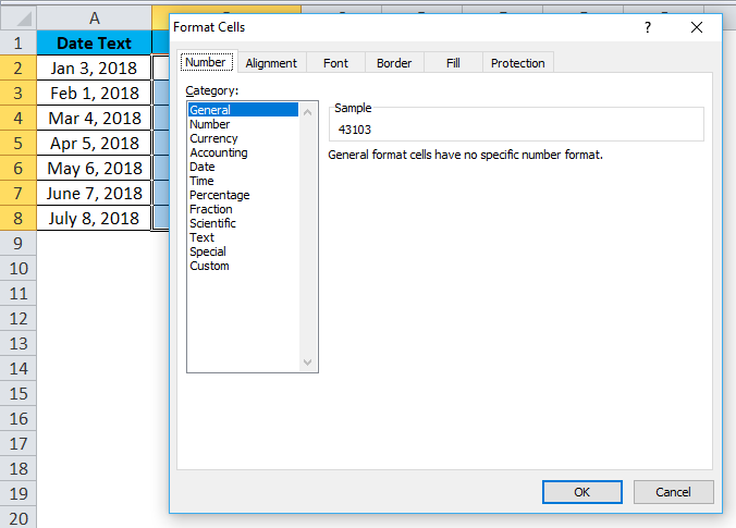
- Click format cells. We will get a list of format options as shown below
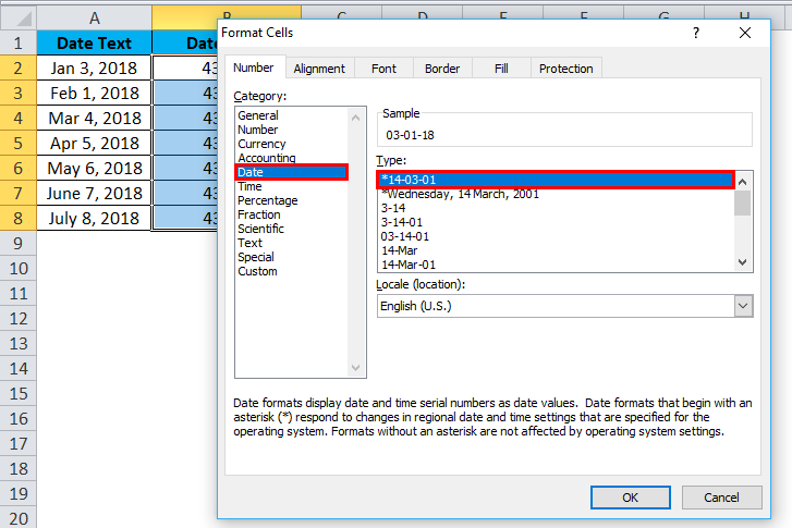
- Choose the appropriate date option by default; Excel will choose the format which has been marked as *
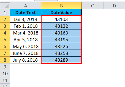
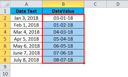
The result is:
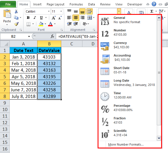
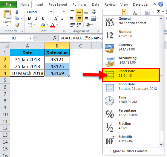
In the advanced version, we have another formatting option where we can find the number tab, as shown in the below screenshot.
- Click on the drop-down box where you will find various formats in the menu bar, as shown below.
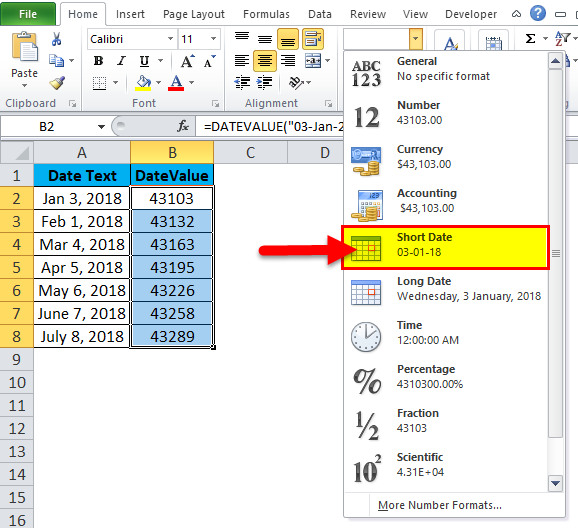
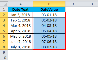
Now choose the date or short date option from the list.
In this way, we can format the cells to get the exact date.
Example #2
We will see various kinds of date formats in which how DATEVALUE WORKS. In the above example, we have seen that we got an error “#VALUE” because the cells are not formatted. DATEVALUE function will work only if the cells are in the proper text format; otherwise, we will get the same error.
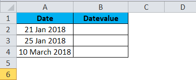
Now let’s consider the below example of how the date value function works. Here in the below example, we can see two columns named date, which is in text format, so to convert to date format, we will use the DATEVALUE function.
Steps to follow for the DATEVALUe function
- Click the insert function in Formula Tab. We will get a dialogue box, as shown below.
- Choose DATE/TIME Category and choose the DATEVALUE function as shown below
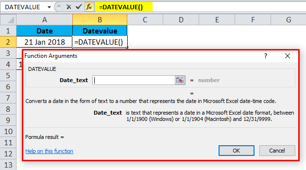
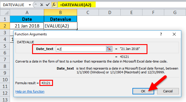
Once we click the DATEVALUE function, we will get the below dialogue box.
Choose the cell to be converted to DATEVALUE and click ok, as shown in the below screenshot.
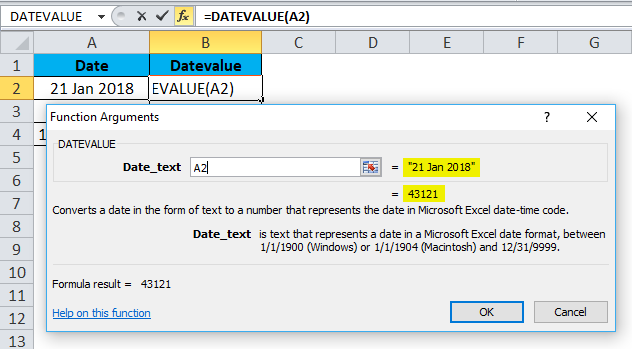
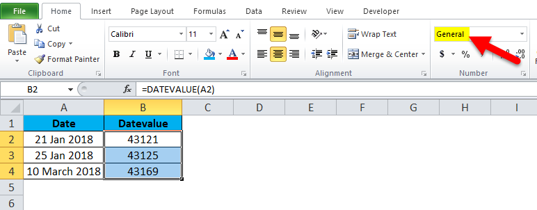
In the below screenshot, we can see that it shows some serial number values as well as a date format on the right-hand side which is highlighted in yellow color.
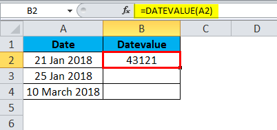
We will get the below result as serial numbers. Where it denotes 21-Jan-2018 is equal to 43121,
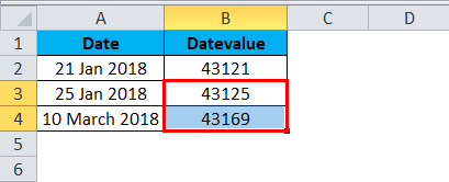
Similarly, we can find the other two.
Here we can wonder why these serial number appears. This is because the specific cells are in the general format, as shown in the below screenshot.
We need to change that general format to the proper date format by choosing a short code from the drop-down box.
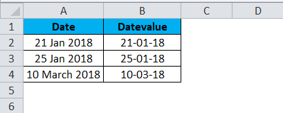
After formatting all the cells, we can see that all serial numbers are converted to the proper date format, shown below as the final result.
Things to Remember
- The first point is it should be in proper text format, then only the DATEVALUE function works.
- We will get the error “#VALUE” if the dates are not in a valid format. So we need to check by formatting the cells to get an exact result.
Recommended Articles
This has been a guide to the Excel DATEVALUE function. Here we discuss the DATEVALUE Formula and how to use the DATEVALUE function in Excel along with practical examples and a downloadable excel template. You can also go through our other suggested articles –

