Updated August 23, 2023
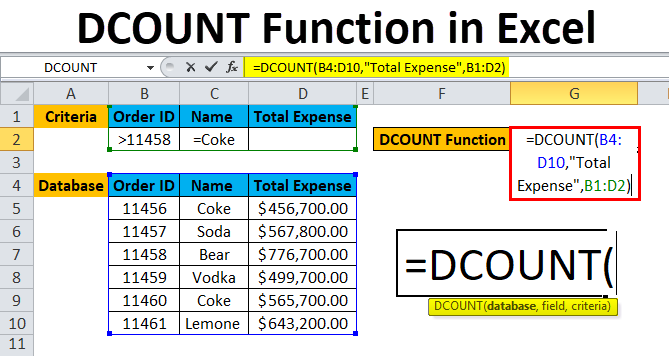
DCOUNT Function in Excel (Table of Contents)
DCOUNT in Excel
The DCount function in Excel is a Database type function which is used to count the cell number, which contains only numbers or numerical values. The selected range for Database in the syntax can be a table or column. Fields part is optional, but here we can select the column whose value we need to count and then for Criteria part range those cell which has criteria. We need to mention the criteria in separate cells by which want cell count.
DCOUNT Formula in Excel
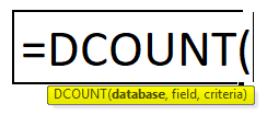
Below is the DCOUNT Formula in Excel :
Below is the component of the DCOUNT function in Excel:
- Database: The Range of cells that the user selected for applying criteria against. The field name must be there in the database. It is a mandatory field.
- Field: The column name or the column number which tell excel which column in the database to count. It will be from the database only. It can be a field number / Index number. It can be omitted the result will be calculated on satisfying criteria.
- Criteria: The range of cells which contain the conditions. The user specifies it. The criteria must contain at least one field name. Criteria can include multiple ranges as the condition specified by the user.
How to Use the DCOUNT Function in Excel?
DCOUNT function in Excel is very simple and easy to use. Let’s understand the working of the DCOUNT function in Excel by some DCOUNT Formula example.
Example #1
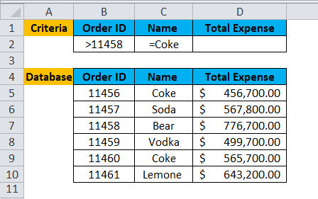
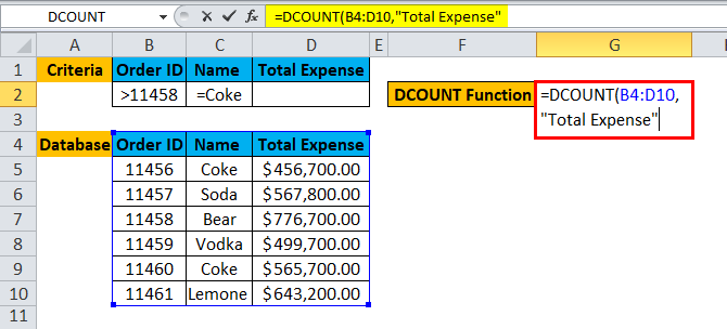
A user wants to calculate the total order made after Order id 11450 for Coke.
Pre-requisite: There is a list of order Id’s, Beverage Name and Expense on a beverage made by some customer. Criteria are written for the same on the top row for which the user wants to count total order.
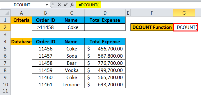
Step 1: Select the G2 cell and write the DCOUNT formula =DCOUNT
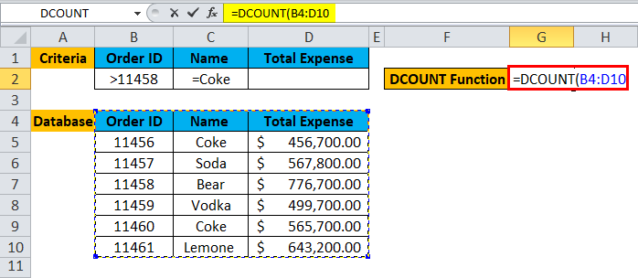
Step 2: Select the database, which is first asked in function, so select B4 to D10.
Step 3: Now enter the field value or column name for which a user wants to count all cell.
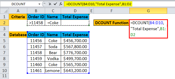
Step 4: Enter the criteria for which the user wants to apply to the database.
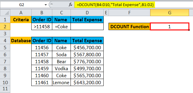
Step 5: Click Enter, the function will be applied to the dataset, and the result will be displayed.
Summary of Example #1:
As we can see from the result, there is only one order: the Order ID is >11458 and Name =Coke.
A user can modify the criteria and can fetch data from the database according to his criteria given to the DCOUNT function in a fraction of seconds.
Example #2
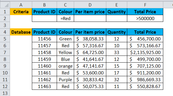
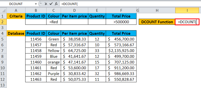
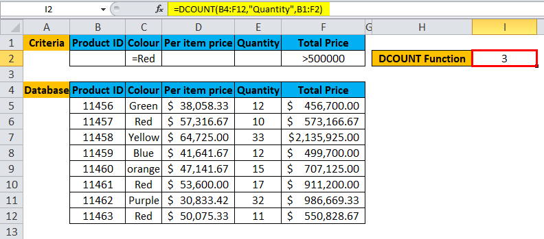
A user wants to calculate the total Product ID, which is Green in color and Price greater than 5 lakhs.
Pre-requisite: There is a list of Product Id, Color description, per item price, quantity and price tag on the product purchased by a customer. Criteria are written for the same on the top row for which the user wants to count total items.
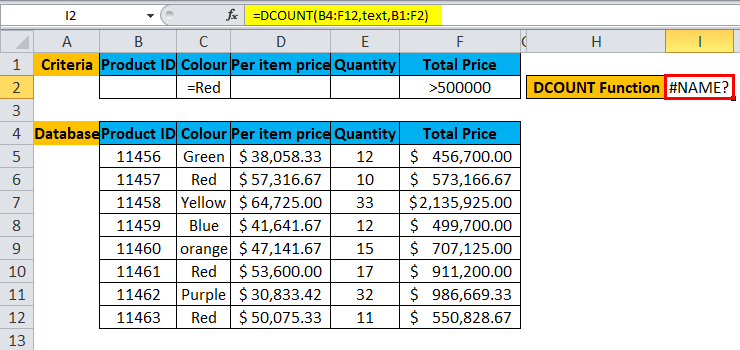
Step 1: Select the I2 cell and write the DCOUNT formula =DCOUNT
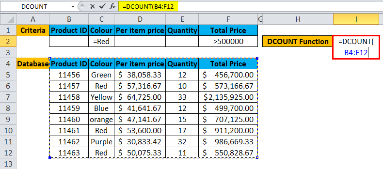
Step 2: Select the database, which is first asked in function, so select B4 to F12.
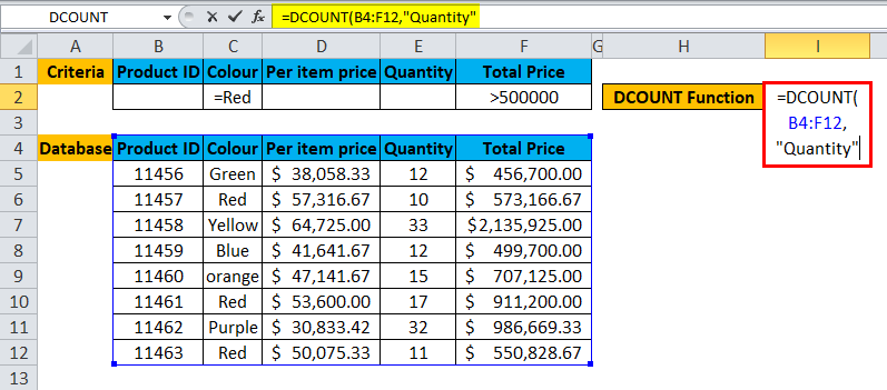
Step 3: Now enter the field value or column name for which a user wants to count all cell.
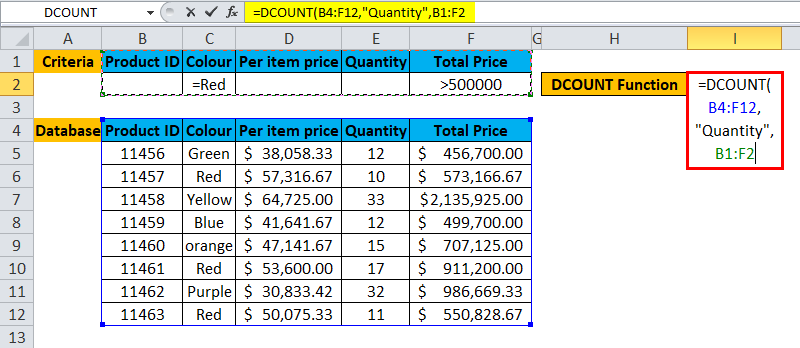
Step 4: Enter the criteria for which the user wants to apply to the database.
Step 5: Click Enter, the function will be applied to the dataset, and the result will be displayed.
Summary of Example #2:
As we can see from the result, there 3 Product ID which color Red and the Total Price is >500000.
A user can modify the criteria and can fetch data from the database according to his criteria given to the DCOUNT function in a fraction of seconds.
Example #3
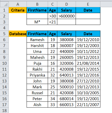
A user wants to calculate the total employee with a salary greater than 6 Lakhs and older than 30 years or whose name starts with the alphabet M and younger than 21 Year.
Pre-requisite: A user has data for some XYZ Company employee data, which have field name like First Name, age, salary and joining date.
Criteria are written for the same on the top row for which the user wants to count total items.
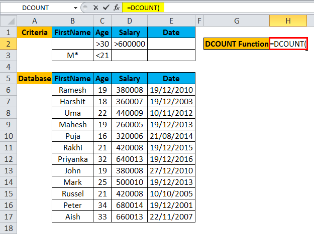
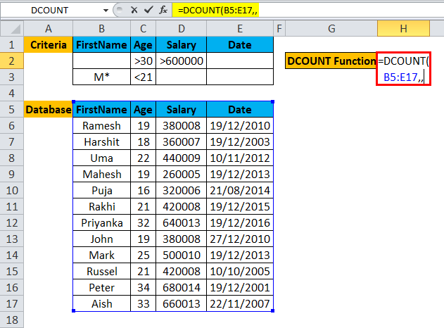
Step 1: Select the H2 cell and write the DCOUNT formula =DCOUNT
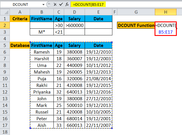
Step 2: Select the entire database, which is first asked in the DCOUNT function, so select B5 to E17.
Step 3: Now DCOUNT function will ask for a field name which we can omit, so a user can skip the field name value and just put a sing comma (,).
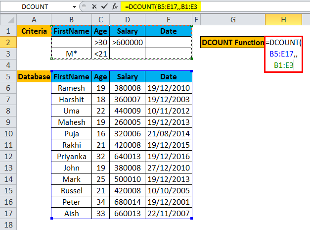
Step 4: Enter the criteria for which user wants to apply on the database, which written on top of the database.
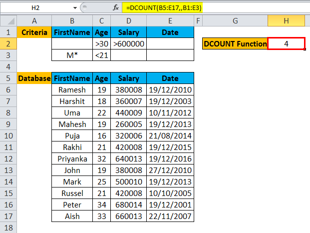
Step 5: Click Enter, the function will be applied to the dataset, and the result will be displayed.
Summary of Example #3:
The user wants to calculate the total employee with a salary greater than 6 Lakhs and older than 30 years or whose name starts with the alphabet M and younger than 21 Year. The same result is displaying in the resultant cell.
A user can modify the criteria and can fetch data from the database according to his criteria given to the DCOUNT function in a fraction of seconds.
A different way to use the DCOUNT function in Excel:
- Field by Name: As we have used in the above example, we have given the field a name.
- Field by Index: A user can give an index name or just a column number.
- Field by Omitted: A user can omit the field value.
Things to Remember About DCOUNT Function in Excel
- DCOUNT function in excel will count only if the user giving non-blank or numeric value. If the field value is blank or text value, then it will throw an Invalid Name Error.
- Criteria can have multiple rows in the DCOUNT function in excel.
- The database and criteria must have the same matching header; otherwise, it will not execute the function.
- The field value can be Name in double quotes (” Name”) or field value index number.
- If criteria in function left blank, then it will throw a #Value error.
- The criteria can be put anywhere in the active sheet. Best to put on top of the database.
- Always make sure the database and criteria or not overlap; there should be at least one-row gap in between.
Recommended Articles
This has been a guide to DCOUNT in Excel. Here we discuss the DCOUNT Formula in Excel and How to use the DCOUNT Function in Excel, along with practical examples and a downloadable excel template. You can also go through our other suggested articles –
