Excel Calculations (Table of Contents)
Introduction to Excel Calculations
The main reason for introducing Excel was to handle day-to-day work calculations, although it is now used for various functions. Like adding, subtracting, multiplication, etc., numbers are used for different purposes for different domains. Though there are other tools for basic calculations, but standoff of using Excel is its flexibility and the perception for the viewer it gives; for instance, we can add two numbers in the calculator as well, but the numbers mentioned in the Excel sheet can be entered in two cells and used for other functions as well subtraction, division, etc.
Let’s have a quick look at some of the calculations to get a better understanding.
How to Calculate Basic Functions in Excel?
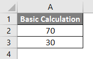
Let us start with the basic calculations and gradually will move further.
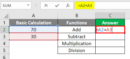
List of calculations that one already knows.
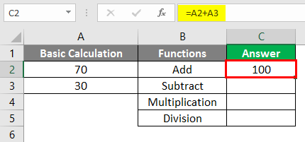
After using the above formula, the output is shown below.
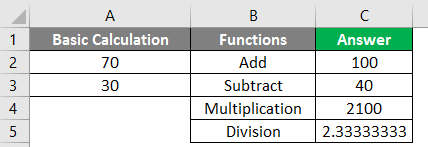
Similarly, a formula is used in cells C3, C4, and C5.
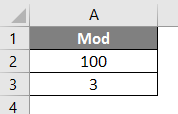
#1 – MOD
Use to get the remainder of two numbers when divided.
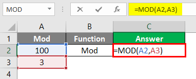
Apply the MOD formula in cell C2.
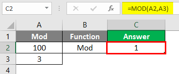
After using the MOD, the Formula output is shown below.
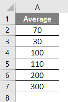
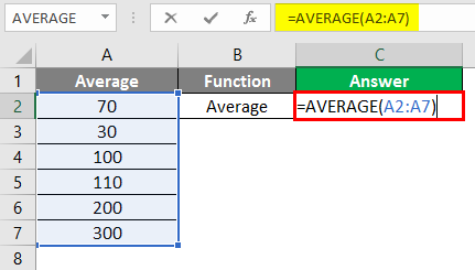
#2 – Average
Use to take the median or average between the range of numbers.
Apply the Average formula in cell C2.
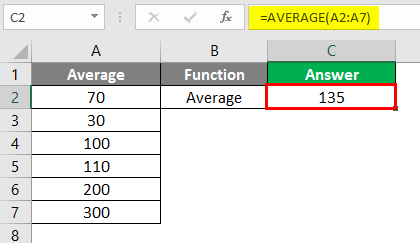
After using the AVERAGE Formula output shown below.
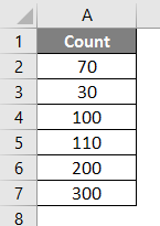
#3 – Count
Use to count the number of cells in data.
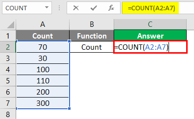
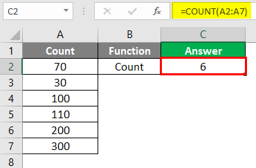
Apply the COUNT formula in Cell C2.
After using the COUNT Formula output shown below.
#4 – Abs
Use for removing the sign from the number
Apply the ABS formula in Cell C2.
After using the ABS Formula output shown below.
#5 – Concatenate
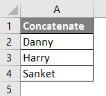
Use for merging text from two or more cells.
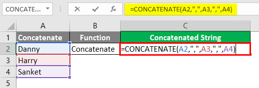
Apply the Concatenate formula in Cell C2.
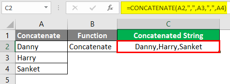
After using the CONCATENATE Formula output as shown below.
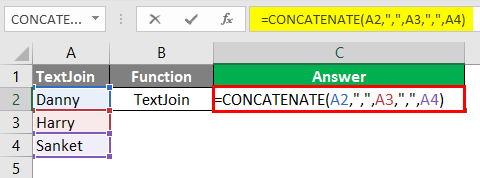
#6 – Text Join
Use for merging text from two or more cells if one has a range; We recommend using this formula, as it may not be available in previous versions.
Apply the Concatenate formula in Cell C2.
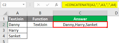
After using the CONCATENATE Formula, the output is shown below.
#7 – IFS
Use instead of IF condition when there are too many conditions to be given, i.e., nested if-else.
Apply the IFS formula in Cell C2.
After using the IFS, the Formula output is shown below.
#8 – VLOOKUP
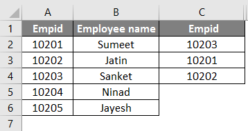
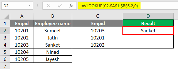
People use the VLOOKUP function in various situations, such as comparing data with one column and validating whether the data is present in the current column. Retrieving the data of the dependent column by comparing the data of the current column with the column on which the dependent column depends; for this, below is an example of one’s preference.
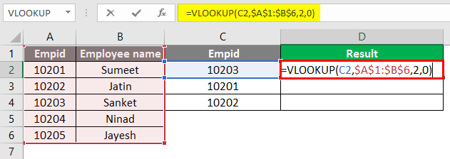
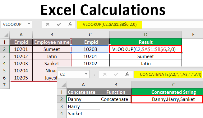
Explanation: The Excel formula compares the “Third column Empid” data with Empid. Based on the Empire, the formula retrieves the corresponding name in the “Result” column.
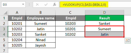
For Example, 10203 from the “Third column Empid” is compared with the “Empid” column, i.e.with 10203, and the corresponding name Sanket is retrieved in the “Result” column.
Apply the VLOOKUP formula in cell C2.
After using the VLOOKUP Formula, the output is shown below.
After using the VLOOKUP Formula, the output is shown below.
#9 – MID
Use for splitting the text or, in easy terms, can be used as a substring.
Apply the MID formula in Cell C2.
After using the MID Formula output shown below.
#10 – LEFT
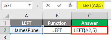
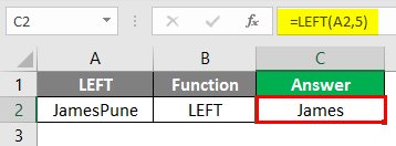
Use the LEFT function when you want to extract characters starting at the left side of the text.
Apply the LEFT formula in cell C2.
After using the LEFT, the Formula output is shown below.
#11 – RIGHT
Use the RIGHT function when you want to extract characters starting at the right side of the text.
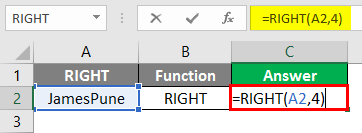
Apply the RIGHT formula in Cell C2.
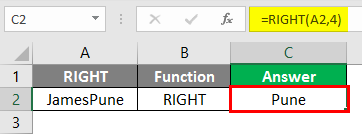
After using the RIGHT Formula, the output is shown below.
Explanation: In the above example, from the text value JamesPune, we only need James, so we use the MID function to split JamesPune to James, as shown in the formulae column. The same goes with a LEFT function, which one can use to split the string from the left side, and the RIGHT function to split the string from the right side, as shown in the formulae.
#12 – FIND
Use for searching the character’s position in the string.
Apply the FIND formula in cell C2.
After using the FIND, the Formula output is shown below.
#13 – LEN
Use for checking the length of the string.
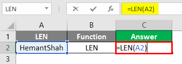
Apply the LEN formula in cell C2.
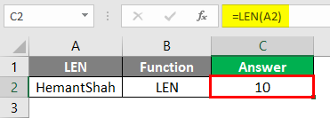
After using the LEN, the Formula output is shown below.
Explanation: The FIND function searches the character’s position in the string like the letter “t” position in the above text is at 6 positions. LEN in the above example gives the length of the string
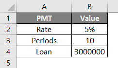
#14 – PMT
It is used for the calculation of monthly installments one has to pay.
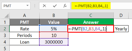
Apply the PMT formula in cell C2.
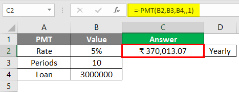
After using the PMT, the Formula output is shown below.
#15 – Nested Formula
Used when our conditions have two to three functions to be used. Suppose we have a text Sau; Mumbai;27 and we want to separate as the Name, then we would go following formula as =MID(A2,1, FIND(“;”, A2,1)-1).
Apply the MID formula in cell C2.
After using the above Formula, the output is shown below.
After using the above Formula, the output is shown below.
After using the above Formula, the output is shown below.
Explanation:
So here for Name, we only want “Sau”, so here we use the combination of MID function, which will help us to split the string, and the FIND function helps to locate the position of; in the string, i.e.as per MID function it needs:
MID(Text_value,start_position, end_position)
Text_value: Sau;Mumbai;27
Start_position: 1
End_position: Position of the first semicolon by FIND function
FIND (find_text, within_text, [start_num])
Find_text = ;
Within_text= Sau;Mumbai;27
Start_num=1
So here, the FIND function gives the position as 4; hence, the MID function looks like this MID(A98,1,4-1). MID(A98,1,3), which would result in “Sau” as shown below Fig:
Pros
- The Excel calculations provide a robust function.
- Calculations can be dynamic.
- Nested Functions are possible.
- More functions add up, helping users ease and avoid more Nested Formulae Example: PMT formula.
Cons
- Nested Formulae become complex to apply.
- Maintaining and using formulas can become challenging if a user is not proficient with Excel.
Things to Remember About Excel Calculations
- Save your worksheet after every application of Excel calculations
- The functions of Excel are increasing daily, so staying updated is important, and avoiding nested formulas is recommended.
- Whenever one applies the function in Excel, one can click on the Tab button to autocomplete the function name, i.e., if one wants to enter a Sum function in a cell, then choose the cell and write “ = S” and press Tab, the function would get autocompleted and, one can also see the value which the function ask for
Recommended Articles
This is a guide to Excel Calculations. Here we discuss How to Calculate Basic Functions in Excel, practical examples, and a downloadable Excel template. You can also go through our other suggested articles –
