Updated May 5, 2023

COLUMNS in Excel

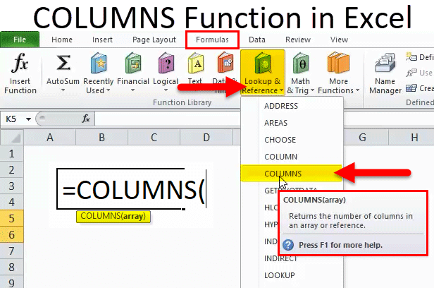
The columns function in Excel is another easiest function to apply, which counts the number of selected columns. It returns the count of the number of columns selected in the array. It will simply return the count of columns there in an array. We must select the complete columns or columns as a table or matrix for this.

COLUMNS Formula in Excel:

The Formula for the COLUMNS Function in Excel is as follows:

The COLUMNS Function formula has the below-mentioned argument:

Array: reference to an array OR range of cells for which we have to calculate several columns.

Note:

Only the columns are counted if the range of cells or array contains multiple rows and columns.
COLUMNS Function in Excel will always return a positive numeric value.

How to Use the COLUMNS Function in Excel?

This COLUMNS Function is very simple and easy to use. Let us now see how to use the COLUMNS Function in Excel with the help of some examples.

You can download this COLUMNS Function Excel Template here – COLUMNS Function Excel Template

Example #1

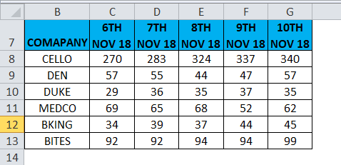
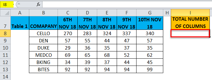
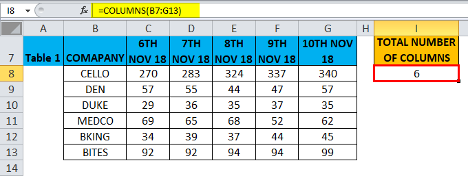
In the below-mentioned example, I have a dataset in a range, i.e., B7:G13, where it contains the company & its share value daily. Here I need to find out the number of columns in that range with the help of the COLUMNS Function.

Let’s apply the COLUMNS function in cell “I8”.

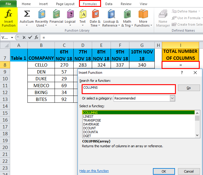
Select the cell “I8” where the COLUMNS function needs to be applied, Click the insert function button (fx) under the formula toolbar, and a dialog box will appear, type the keyword “COLUMNS” in the search for a function box, COLUMNS function will appear in select a function box.

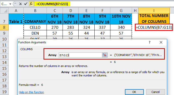
Double click on the COLUMNS function, and a dialog box appears where arguments for the COLUMN function need to be filled or entered, i.e., =COLUMNS (array)

Array: Reference to an array OR range of cells for which we have to calculate several columns, i.e., Here it is B7:G13, where B7 is a starting cell, and G13 is the ending cell in a table or range.

Click ok after entering the arguments in the COLUMNS function. i.e.=COLUMNS (B7:G13) COLUMNS function calculates the total number of columns present in a range, i.e., 6. The number of columns between these two cells (B7 & G13) is 6, resulting in 6.

Example #2

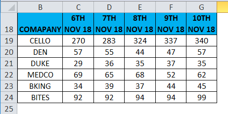
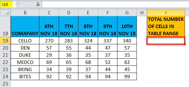
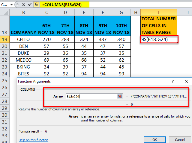
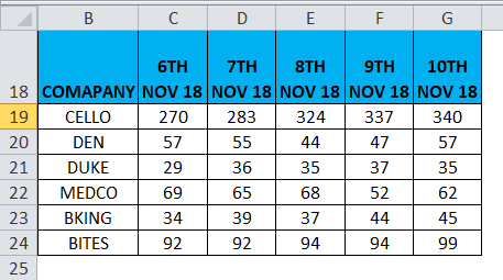
In the below-mentioned example, I have a dataset in a range, i.e., B18:G24, where it contains the company & its share value daily. Here I need to find out the Total cell in range with the help of the COLUMNS function.

Let’s apply the COLUMNS function in cell “I19”.

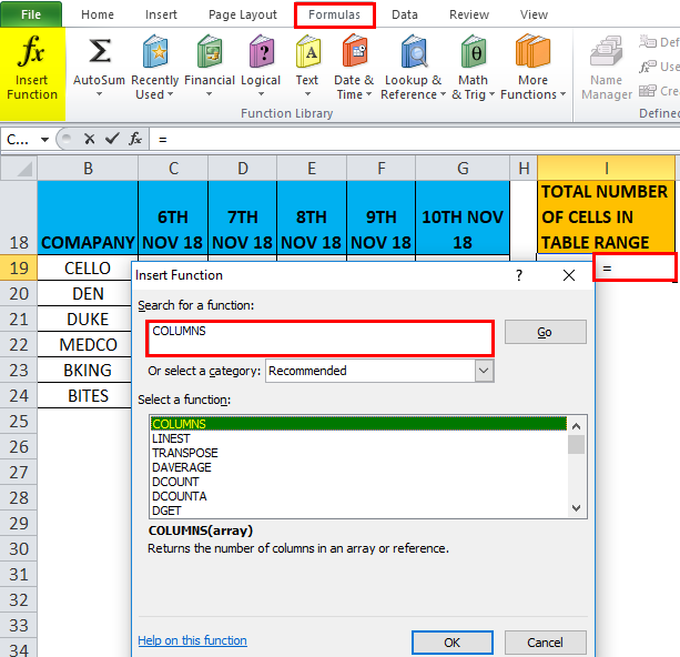
Select the cell “I19” where the COLUMNS function needs to be applied, Click the insert function button (fx) under the formula toolbar, and a dialog box will appear, type the keyword “COLUMNS” in the search for a function box, COLUMNS function will appear in select a function box.

Double click on the COLUMNS function, A dialog box appears where arguments for the COLUMN function need to be filled or entered i.e.

=COLUMNS (array)

Array: reference to an array OR range of cells for which we have to calculate a number of columns, i.e., here it is B18:G24 where B18 is a starting cell, and G24 is the ending cell in a table or range.

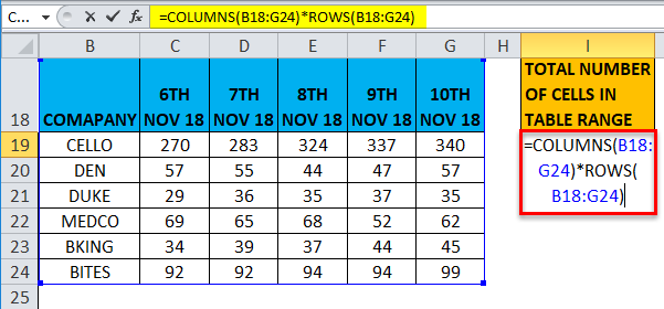
Multiplication must be performed between the total number of columns and a total number of rows for the given array or range of cells to get the total number of cells in an array or table.

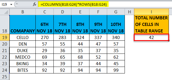
i.e. =COLUMNS(B18:G24)*ROWS(B18:G24)

Here, the total number of rows is 7 & the total number of columns is 6. So, the total number of cells is 7*6 = 42

Example #3

The COLUMNS function is important when using functions where a column argument is required, e.g., VLOOKUP, in case of a huge number of datasets; it is not easy to manually count the number of columns in a table array.

During these scenarios, In the VLOOKUP function, The COLUMNS function is used to return the col_index_num argument value.

Let’s check out the difference between the Vlookup function with & without Columns Function.

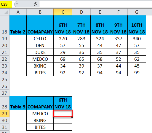
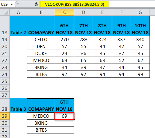
In the below-mentioned example, table 2 contains the company in column B & its share value on a daily basis ( 6^th, 7^th,8^th, 9^th & 10th Nov 2018) in columns C, D, E, F & G, respectively.

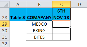
Table 3 contains the company name in column B; our objective here in this table is to find out its share value on 6^th Nov 2018 in column C, with the help of table 2 reference by using the VLOOKUP function.

Before applying the VLOOKUP formula, you should be aware of it. Vertical lookup or VLOOKUP references vertically aligned tables and quickly finds data in relation to the value the user enters.

VLOOKUP Function without COLUMNs Function

Let’s apply the VLOOKUP function in cell “C29”.

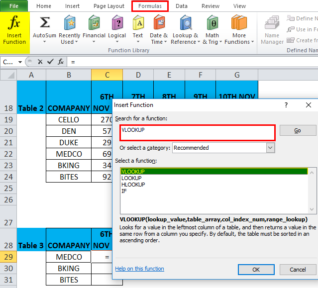
Select the cell “C29”. where the VLOOKUP function needs to be applied; click the insert function button (fx) under the formula toolbar, and a dialog box will appear, type the keyword “VLOOKUP” in the search for a function box, VLOOKUP function will appear in select a function box.

Double click on the VLOOKUP function, A dialog box appears where arguments for the VLOOKUP function must be filled or entered.

The Formula for the VLOOKUP function is:

VLOOKUP (lookup_value, table_array, col_index_num, [range_lookup])

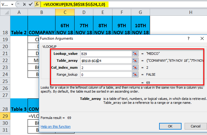
lookup_value: The value you want to look up, i.e., “B29” or “MEDICO.”
table_array: Range where the lookup value is located, i.e., select table 2 range B18:G24 & click function f4 key to lock a range, i.e., $B$18:$G$24.
col_index_num: column number in a table array from which the matching value should be returned. Here the company share value on 6^th November 2018 is in Table 2 & it is in the second column, i.e., 2
range_lookup: FALSE for an exact match or TRUE for an approximate match. Select 0 or false.

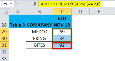
=VLOOKUP(B29,$B$18:$G$24,2,0) returns the share value of Medco on 6^th November 2018, i.e. 69

To get the finalized data for other company share prices, click inside cell C29 to see the cell selected, then Select the cells until C31. So that the column range will get selected. Once it got selected, click on Ctrl + D to apply the VLOOKUP formula to a whole range.

VLOOKUP Function with COLUMNS Function

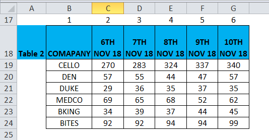
Above the Table 2 column header, B17 to G17 is the column number that needs to be mentioned before applying Vlookup with the columns function.

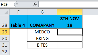
Table 4 contains the company name in column G; our objective here in this table is to find out its share value on 8^th Nov 2018 in column H, with the help of table 2 reference by using VLOOK with COLUMNS function.

In VLOOKUP Function without COLUMNS Function, Formula was:

=VLOOKUP(C29,$B$18:$G$24,2,0)

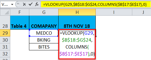
Where 2 was the column index number, let’s replace this with the COLUMNS($B$17:$E$17) function in the Vlookup function in cell H29 of Table 4. Here we need a share price value for 8^th Nov 18, hence the select column reference B17 to E17 in the columns function of the table.

i.e. =VLOOKUP(G29,$B$18:$G$24,COLUMNS($B$17:$E$17),0)

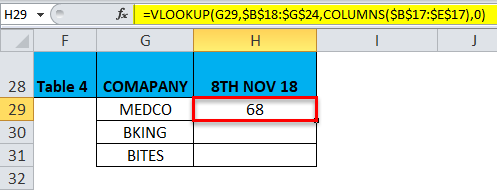
=VLOOKUP(G29,$B$18:$G$24, COLUMNS($B$17:$E$17),0) returns the share value of Medco on 8^th November 2018, i.e. 68

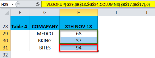
To get the finalized data for other company share prices, click inside cell H29 to see the cell selected, then Select the cells till H31. So that the column range will get selected, once it is selected, press Ctrl + D so that the formula is applied to a whole range.

Here simultaneously, we have to change the column reference in the column function & lookup value based on the data requirement.

Things to Remember

The COLUMNS Function in Excel is significant when using functions where a column argument is required (e.g., VLOOKUP); in the case of a huge number of datasets, it is not easy to manually count the number of columns in a table array (Explained in example 3).
The array argument in the COLUMNS Function can be either a range of cells or single-cell addresses.
Only the columns are counted if the range of cells or array contains multiple rows and columns.
COLUMNS function in Excel will always return a positive numeric value.

Quiz Result
Total Questions	Correct Answers	Wrong Answers	Percentage

COLUMNS in Excel