Date Format in Excel
You can choose how you want to write your dates using “Date Format in Excel.” The Date Format does not change the actual date itself; it only changes how you write it. It means you can tell Excel to show the date in a way that makes sense.
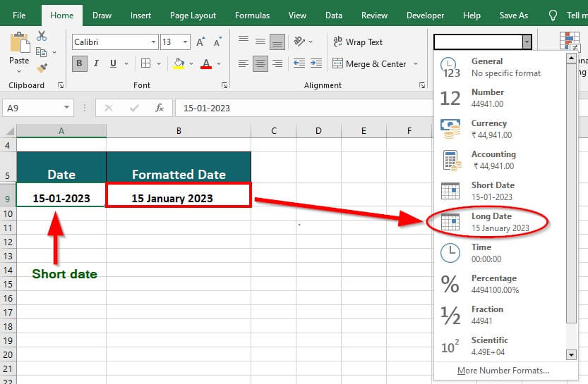
For example, if you want to see the month spelled out like “May” instead of “05“, you can change the format. You can also use it to convert a short date, such as 15-01-2023, into a long form as 15 January 2023.
Excel date formats enable users to perform various calculations, such as adding and subtracting dates, finding the difference between two dates, and determining the average of a range of dates. Additionally, practicing with Microsoft MS-102: Practice Test Dumps can help users gain a deeper understanding of managing date formats, functions, and other Excel-related tasks for improved efficiency.
How Excel Stores Dates?
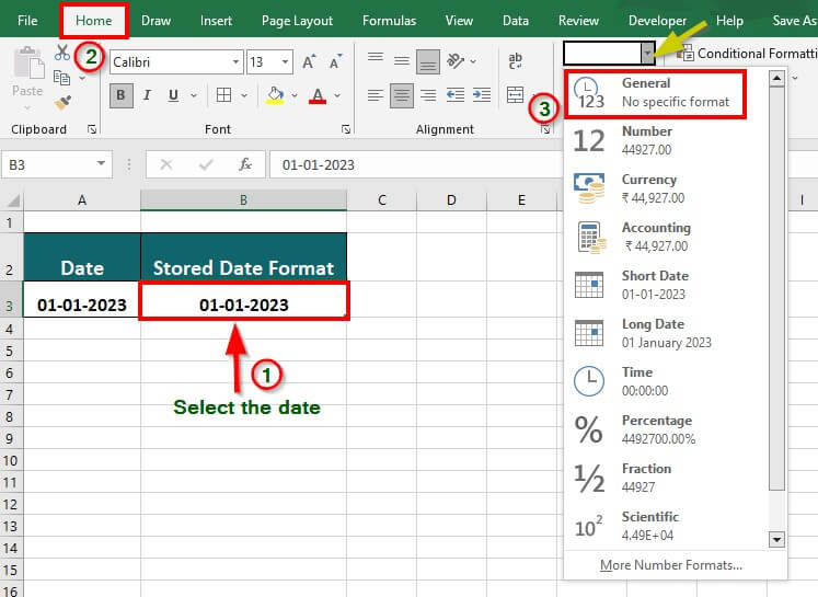
Microsoft Excel stores data in a numerical format to use for calculations. To explore how Excel stores a date, follow these steps:
Step 1: Select the cell containing the date
Step 2: Go to the Number group in the Home tab.
Step 3: Select General from the drop-down menu
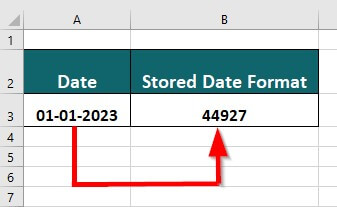
As illustrated below, it converts your chosen data into an integer format.
The below image shows the integer value for the given date.
The date serial number 44927 tells us how many days it has been since 1st January 1900.
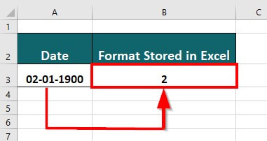
Excel gives the number series for the dates from 1 Jan 1900 to 31 Dec 9999. It means Excel stores 1 Jan 1900 as the integer value 1, 2 Jan 1900 as the integer value 2, and so on. To check this, you can follow the same procedure of converting the data into a General format. The below image shows the output.
How to Change Excel Date Format?
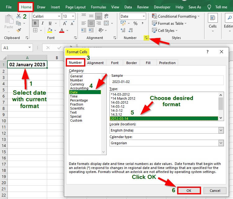
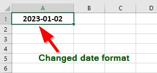
To change the date format in Excel, follow these steps:
Step 1: Select the cell containing the date with the current format
Step 2: Navigate to the Number group in the Home tab.
Step 3: Click on the list arrow to open the Format Cells dialog box
Step 4: Go to Date in the Number tab in the Format Cells window.
Step 5: Select the Locale (location) from the drop-down list.
Step 6: Select the desired Excel date format from the Type list.
Step 7: Click OK.
Let us understand how we can change a date format using different methods, along with some illustrative examples.
Example #1: Display Given Date in Long Form
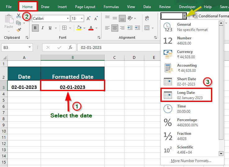
Here are the steps to convert and display a given date in a long form:
Step 1: Select the cell containing the date and go to the Home tab
Step 2: Select Long Date from the Number group drop-down menu.
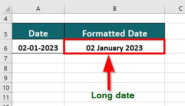
It converts and displays the given date into a long form, as shown in the image below.
Example #2: Change Excel Date Format Using the “Custom” Option
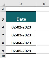
Consider the following dates that require a format conversion using the Custom option.
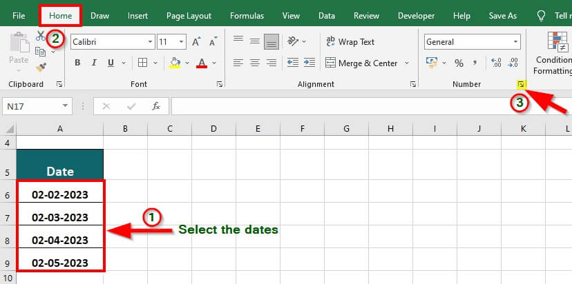
Step 1: Select the cells containing the dates.
Step 2: Navigate to the Home tab, then select the list arrow in the Number group.
A Format Cells window opens up.
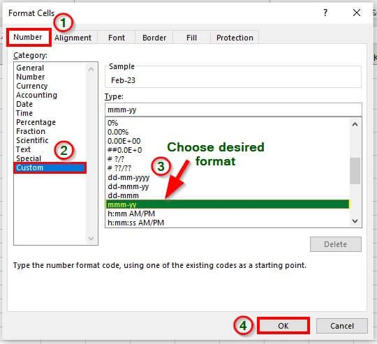
Step 3: Click the Number tab and select Custom from the Category list.
Step 4: Choose the desired date format from the Type field.
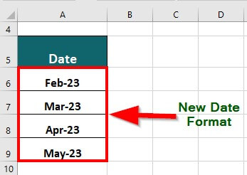
In this case, we choose the format “mmm-yy“, representing month and year
Step 5: Click OK.
Excel converts the dates accordingly and showcases the output in the image below.
If you wish to modify the Default Date settings, follow these steps:
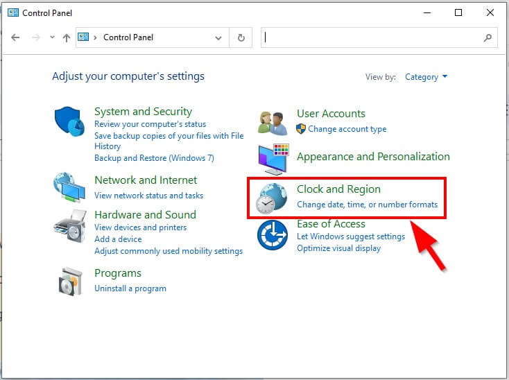
Step 1: Locate the Control Panel and click Clock and Region.
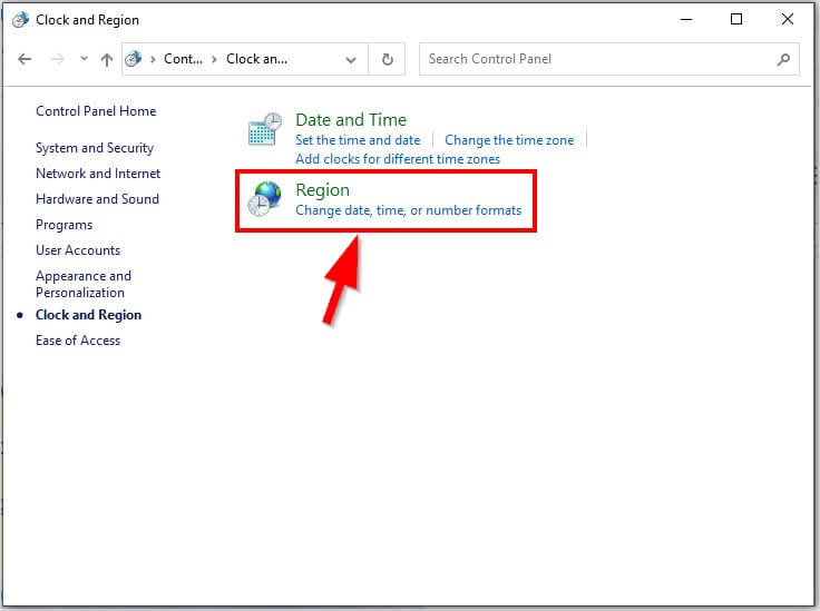
Step 2: Click Region.
It opens a Region window with different settings.
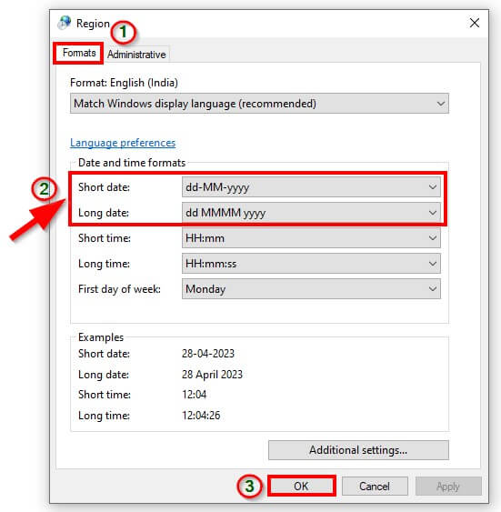
Step 3: Click Formats and choose the desired date format from the Short Date and Long Date drop-down list.
Step 4: Click OK.
Example #3: Using Date with the COUNTIF Function in Excel
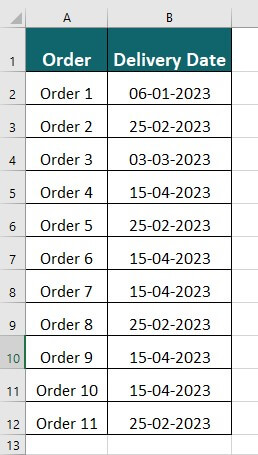
Let us consider a scenario where a courier company has a list of orders and aims to determine the number of orders it delivers on a specific date, such as February 25, 2023, using the COUNTIF function in Excel.
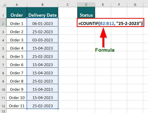
Step 1: Enter the following formula: =COUNTIF(B2:B12, “25-2-2023”) in an empty cell (Cell D2).
The formula will determine the count of cells within the specified range (B2:B12) that comprise the date “25-2-2023”.
Step 2: Press Enter key.
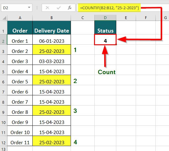
Step 3: In this case, the number of occurrences of “25-2-2023” in the range (B2:B12) is 4. Therefore, the formula gives the output as 4.
Example #4: Finding the Difference Between Dates using the DATEDIF Function
Suppose you have a list of dates and desire to compute the duration/ difference between them in terms of the number of days, months, and years utilizing the DATEDIF function in Excel.
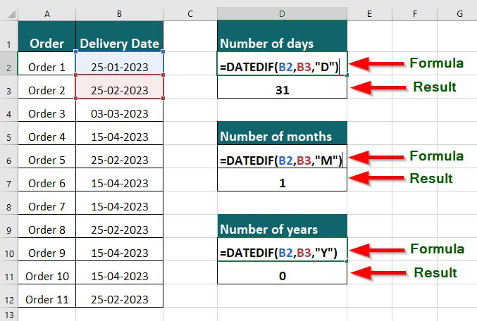
The syntax for the number of days is =DATEDIF(start_date,end_date,” D”).
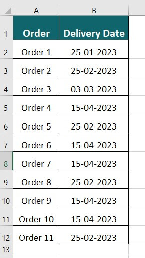
Assuming the start date is 25-01-2023 and the end date is 25-02-2023.
Step 1: In an empty cell (Cell D2) enter the formula =DATEDIF(B2,B3,”D”)
The formula counts the total number of days present between 25-01-2023 and 25-02-2023, including the end date. Since the difference between the two dates is 31 days, the formula yields a result of 31.
The syntax for the number of months is =DATEDIF(start_date,end_date,”M”)
Step 2: In an empty cell (here, cell D6), enter the formula =DATEDIF(B2, B3,” M”)
The formula counts the total number of months between 25-01-2023 and 25-02-2023, including the end date. There is a difference of one month between the given dates; therefore, the formula gives the output of 1.
The syntax for the number of years is =DATEDIF(start_date,end_date,” Y”).
Step 3: In an empty cell (Cell D10) enter the formula =DATEDIF(B2,B3,”Y”)
The formula counts the total number of years present between 25-01-2023 and 25-02-2023, including the end date, and gives the result of 0.
The below image illustrates the above example.
Things to Remember
- Excel can only recognize and convert dates that begin from 1 Jan 1900. Therefore, all dates before it remains in the same format even if you try to change them.
- Excel displays a negative date as #######. Thus, ensuring that you provide positive date values when working with the 1900 date system is essential.
- Excel represents the default date with the “*” symbol specified in your system’s control panel.
- The shortcut to display the current date is “CTRL +;” (You must press Ctrl and Semicolon keys together)
- Excel treats date as numbers; therefore, using functions while calculating dates is essential for accurate results.
- For instance, you can use the NETWORKDAYS function to calculate the number of working days between two given dates, which considers weekends and holidays.
Frequently Asked Questions (FAQs)
Q1. What is the common Excel date format?
Answer: The most common Excel date format we use is dd/mm/yyyy.
- dd- represents the day
- mm- means the month
- yyyy- represents the year
Q2. What is the easiest way to change the date format in Excel?
Answer: To quickly change the Excel date format, follow these steps:
Step 1: In the Home tab, go to the Number group.
Step 2: Click on the list arrow to open the Format Cells dialog box
Step 3: Go to Date in the Number tab in the Format Cells window.
Step 4: Choose the desired country’s date format from the Locale(location) drop-down list.
Step 5: Select the desired date format from the Type list.
Step 6: Click OK.
Q3. What are the main date formats?
Answer: Different regions and languages often use different date formats, and it’s essential to be aware of these differences when communicating with people from other places.
1. English-speaking countries: The most common date format is M-D-Y (mmmm-dd-yyyy), which means we first write the month, then the day, followed by the year.
Example: We can write February 9th, 2023, as 02-09-2023 or February 9, 2023.
2. French-speaking countries: The most common format is D-M-Y(dd-mmmm-yyyy), which means the day is written first, followed by the month, and then the year.
Example: February 9th, 2023, would be written as 09-02-2023 or 9 février 2023.
Recommended Articles
This has been a guide to Date Format in Excel. Here we discussed How to change the Date Format in Excel, practical examples, and a downloadable Excel template. You can also go through our other suggested articles –
