Updated August 11, 2023
Freeze Rows in Excel
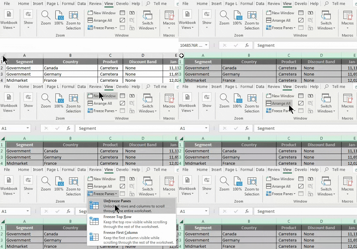
In Excel, we have a function for freezing the rows as well. With the help of Freeze Row, we can fix the pane or row we select to go beyond the certain limit worksheet. Freeze Row can be accessed from the View menu tab’stab’s Window section from the drop-down list of Freeze Panes. First, to freeze the column, select the column we want to freeze, put the cursor anywhere in that column, and then select the Freeze Column option from the list. We will be able to see the selected column is now frozen.
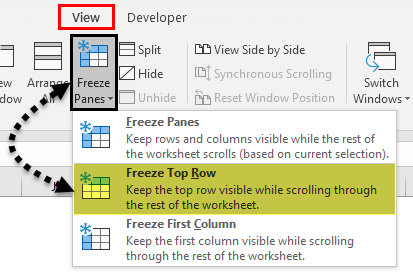
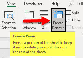
The freeze option is located under the View tab in Excel.
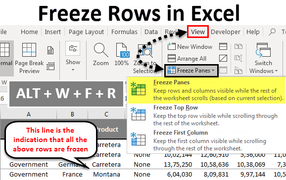
Here we have 3 options. Freeze Panes, Freeze Top Row, and Freeze Top Column. I will show you examples of Freeze Rows in this article.
How to Freeze Rows in Excel?
We use Freeze Panes in Excel to keep an area or heading of a worksheet visible while scrolling to another part of a worksheet. This is very useful and convenient when working on a large table. So we select Freeze Panes from the View tab and keyboard shortcuts to lock that area.
Let’s understand how to Freeze Panes in Excel with some examples.
Freeze or Lock Top Row – Example #1
Usually, our header is located in each column, i.e., horizontally. When scrolling down, we need to lock or freeze our first or top row, enabling us to see the first or top row at any given time.
Now look at the below image of sales data in the sheet.
It isn’t easy to see all the headers when scrolling down. So, in Excel, we have an option called Freeze Top Row, which holds onto the top row when scrolling down and helps us see the heading all the time.
Let’s look at the below steps to understand the method.
Step 1: Select the worksheet where you want to freeze your top row.
Step 2: Go to VIEW tab > Freeze Panes > Freeze Top Row.
We have a shortcut key as well. Press ALT + W + F + R.
Step 3: Ok, done. It is as easy as you eat pizza. You have frozen your top row to see the top row while scrolling down.
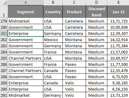
Even though I am in the 281st row, I can still see my headers.
Freeze or Lock Multiple Rows – Example #2
We have seen how to freeze the top row in the Excel worksheet. I am sure you found it a walk-in-the-park process; you did not have to do anything special to freeze your top row. But we can freeze multiple rows as well. So here, you need to apply simple logic to freeze multiple rows in Excel.
Step 1: Identify how many rows you need to freeze in the Excel worksheet. For an example, take the same data from the above example.
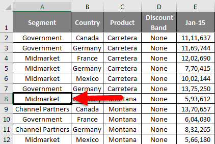
Now I want to see the data of the product Carretera, i.e., from C2 cell to C7 cell all the time. Remember that I don’t just want to see the row but to see the product and compare it with others.
Place a cursor on the A8 cell. This means I want to see all the rows above the 8th row.
Step 2: Remember we are not only freezing the top row, but we are freezing multiple rows at a time. Do not press ALT + W + F + R in a hurry; hold on momentarily.
After selecting cell A8 under freeze panes, again select the option Freeze Panes under that.
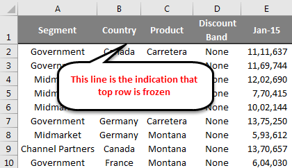
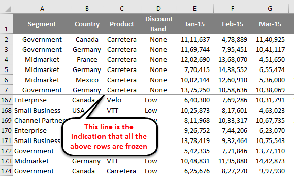
Now we can see a tiny grey straight line below the 7th row. This means the above rows are locked or frozen.
You can keep seeing all 7 rows while scrolling down.
Things to Remember
- We can freeze the middle row of the Excel worksheet as your top row.
- Make sure the filter is removed while freezing multiple rows at a time.
- If you place a cursor in the unknown cell and freeze multiple rows, then you may go wrong in freezing. Make sure you have selected the right cell to freeze.
Recommended Articles
This has been a guide to Freeze Rows in Excel. Here we discussed How to Freeze Rows in Excel and different methods and shortcuts to Freeze Rows in Excel, along with practical examples and a downloadable Excel template. You can also go through our other suggested articles to learn more –
