Updated August 9, 2023
Excel Function for Range (Table of Content)
Range Function in Excel
Range in Excel is the difference between the maximum and minimum limits of the available numbers in Excel. For example, around 10 different numbers are randomly selected in a list in Excel.
To calculate the Range for these numbers, we need to find the upper and lower values using the MAX and MIN functions in the list of those cells. Once we get the maximum and minimum values out of those numbers, subtract the Max value from the Min value. The returned number will be the range.
There are two kinds of ranges used extensively in Excel, which are illustrated below:
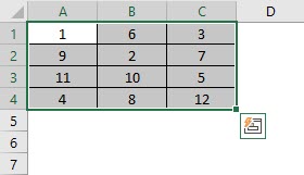
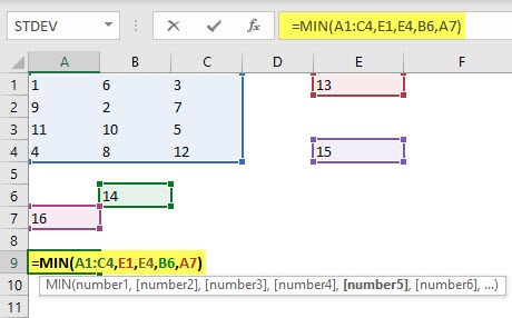
Symmetrical Range: A range that consists of all cells in adjacent positions to each other. Such a range usually shows up as a square or rectangle in a spreadsheet when highlighted. The range shown in the image would be (A1:C4)
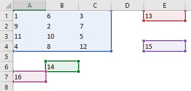
Irregular Range: A range consisting of cells that are not contiguous and may not have regular geometrical shapes when highlighted. The range highlighted in the image would be (A1:C4, E1,E4, B6,A7)
Examples of Range Function in Excel
Now, a range would be useless as we have to derive insights from the range’s data. So formulae are used with cell ranges which add the operation we want to perform in the data from the range. For example, if we want to find the sum of the numbers in cells A1 to C4, we would use =SUM(A1:C4)
Example #1 – Finding Maximum and Minimum
1) Finding the maximum and minimum values in a cell range: We use the following functions when looking for minimum and maximum values in a cell range. Please note that this would give us the mathematical result, not the maximum and minimum, as defined by cell number.
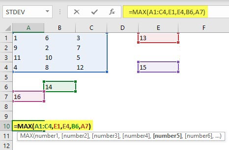
- For Maximum: As illustrated below, we would use the =MAX(Cell Range) function.
- For Minimum: We would use the =MIN(Cell Range) function as shown below.
2) Suppose we are not interested in the minimum and maximum in the highlighted range but also in the top and bottom k numbers. We can use the following functions to calculate those.
- For the top k number, say k=3, which means the third-largest number in the range, we would use the function =LARGE(Cell Array,k) for symmetrical ranges or =LARGE((Cell Range),k) for irregular ranges as shown below.
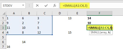
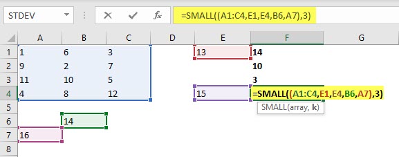
- A very similar function for finding the kth smallest number in a range would be to use =SMALL(Cell Array, k) for a symmetrical range or =SMALL((Cell Range),k) for an irregular range.
Example #2 – How to Define and Use Ranges in Excel?
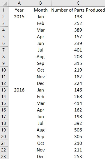
We will now look at how to define and use ranges in Excel. First, we need to have data to work with. This can be anything in a spreadsheet ranging from letters to numbers or a combination of both. For the illustrations accompanying this discussion, I am using a sample from a production database that stores data on how many parts are produced in a year.
Let us say we want to know the range of production numbers entered over the two years. We do this by subtracting the minimum from the maximum value. For this, we need not find each value individually but have to break down the calculation steps and write the formula as follows:
MAX(Cell Range)-MIN(Cell Range)
Please note that the cell range has to be the same in the arguments; otherwise, the formula will not return the correct result.
We find that the range of products is 368 parts. Now, if we want to find out the occurrence of a particular value in the range, or a range of values within the range, we use another function called COUNTIF. This function has the following syntax:
COUNTIF(Range, value)
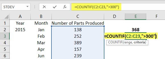
Suppose we want to find the month in which we hit more than 300 parts. The formula would be =COUNTIF(C2:C23,”>300″)
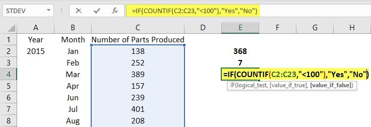
We find that for 7 months, the production was more than 300 parts. We can also find out if we had any month below a particular number, suppose 100. We would use a nested COUNTIF formula within an IF statement to get a Yes or No answer like this:
=IF(COUNTIF(range,” value”),” Yes”,” No”)
This would look like this:
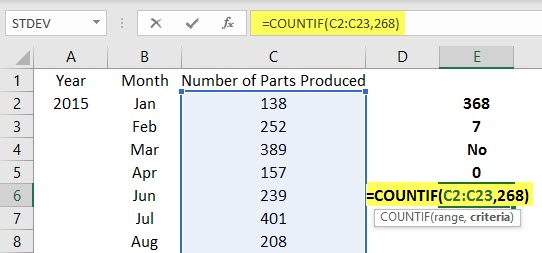
The result would be a No as none of the production numbers in the range is below 100. A variation of this can be used to find if we have any production number in a particular value. This would be as follows:
COUNTIF(range,”*”&value&”*”) or COUNTIF(range, value)
The first variation is useful if we want to match two different databases, and the second is when we want to find out if a particular value occurs or not, and if it does, then how many times it reoccurs.
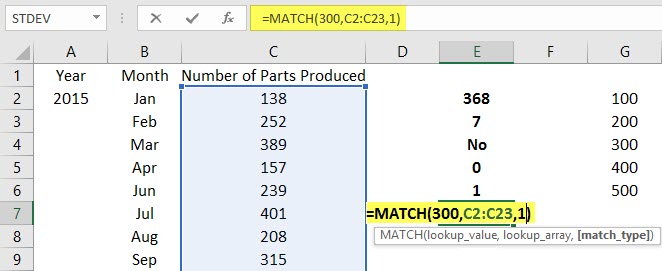
We can use the MATCH function instead of COUNTIF to find the number of values greater or less than a given value.
In the above example, we use the MATCH function to find the number of months with less than 300 parts produced.
Things to Remember
- We should sort the data in ascending or descending order wherever feasible to simplify operations using ranges.
- Quotation marks (“”) and asterisks (*) are used in formulae whenever we are looking for substrings or specific text ranges within a range.
- Irregular ranges are the most common ranges used in business. As such, whenever possible, we should use tables to classify the data before running any operations on them.
- It must be noted that ranges can be highlighted manually, and Excel displays the number of cells in it as a count at the bottom; however, we can find out the number of rows or columns in a range using the following functions:
ROWS(range)
COLUMNS(range)
Usually, these two functions are not required but are useful for large tables, multiple databases, and recording macros.
Conclusion
Knowledge of range in Excel is an important prerequisite to manipulating data. The range is also used in recording macros and VBA coding; hence, an in-depth understanding of range is necessary for anyone using Excel.
Recommended Articles
This is a guide to Excel Function for Range. Here we have discussed Examples of Range Functions in Excel, along with steps and a downloadable Excel template. You may also look at the following articles to learn more –
