Updated August 23, 2023
LARGE Function in Excel
A large function in excel is an inbuilt statistical function that returns the nth position or Kth position from the selected numerical array. If the Kth position is greater or larger than the values, there is an array, or if we keep the Kth position blank, it will return #Num! As error. This means while putting the Kth value in the syntax, we need to put the value which is the lowest number from the selected array or any lowest number, but it should not be in an array.
This function can sort the information provided and find the maximum value.
LARGE Formula in Excel
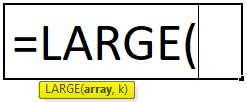
Below is the LARGE Formula:
Where the passing arguments are:
- Array–the array or range of data from which we want to select the largest value.
- K – An integer value specifies the position from the largest value.
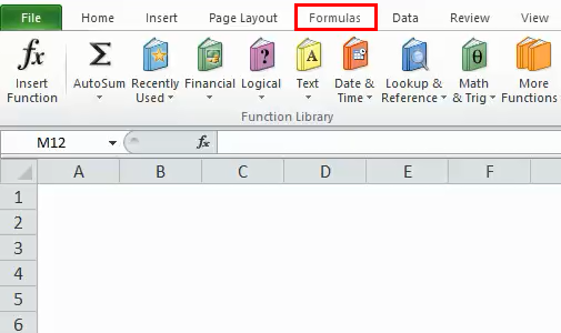
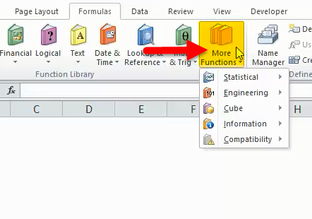
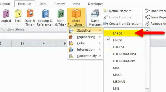
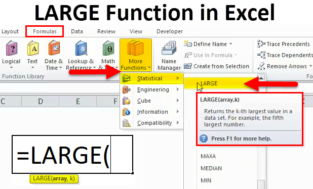
As the LARGE function falls under the Statistical function category, and it is a built-in function in Excel, i.e. this function can be found under the FORMULAS tab in Excel. The steps are as follows:
- Click on the FORMULAS tab.
- Click on the More Functions tab.
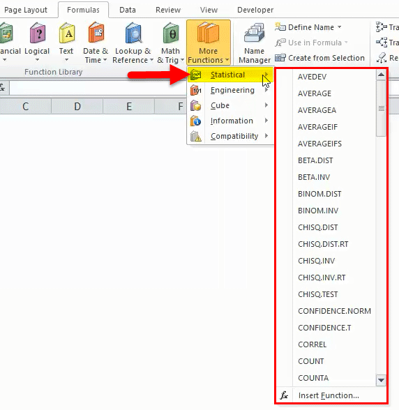
- Select the Statistical functions category. It will open the drop-down list of functions.
- Click on the LARGE functions tab from the drop-down list.
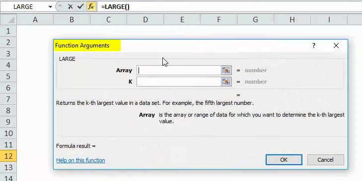
- After selecting the LARGE function, a Function arguments box will pop up.
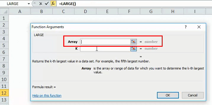
- Enter the Array field with an array or range of data you want to find the nth largest value.
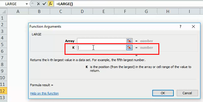
- Enter the K field; it is the position from the largest value in the array of the value to return.
How to use the LARGE Function in Excel?
LARGE Function is very simple to use. Let us now see how to use a LARGE function with the help of some examples.
Example #1
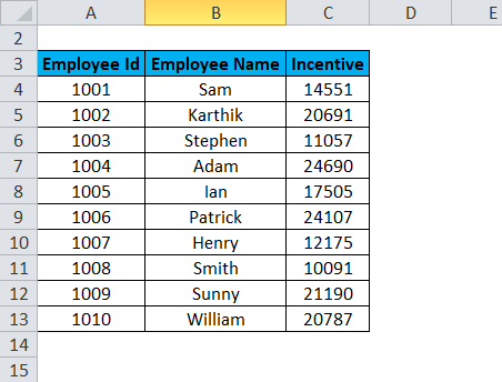
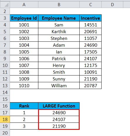
Suppose we have company employee data, and the company distributes incentives to their employees based on their performance. We need to find out the name of the employees who are in the top 3 on the list and received the highest incentives.
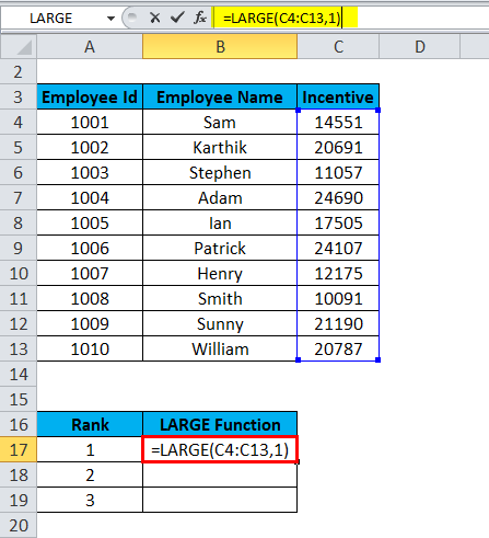
To find the employee name who has achieved the largest incentive, will use the below formula:
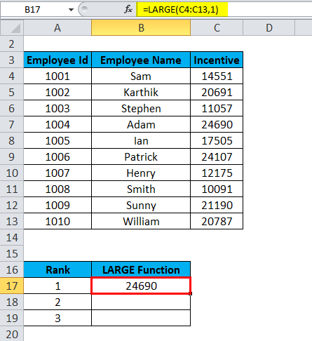
=LARGE(C4: C13,1)
The Result is:
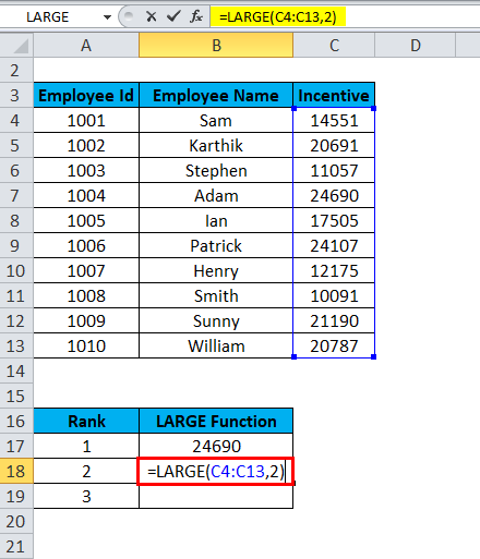
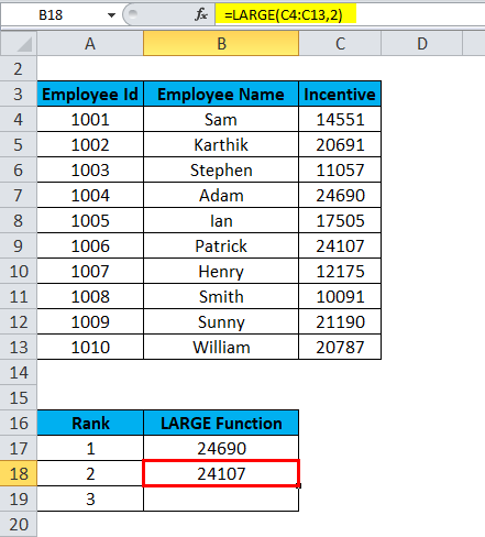
To find the employee name who has achieved the second-largest incentive, will use the below formula:
=LARGE(C4: C13,2)
The Result is:
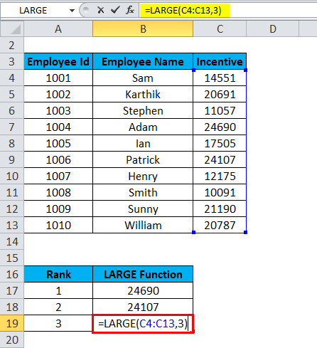
To find out the employee name who has achieved the 3rd largest incentive, will use the below formula:
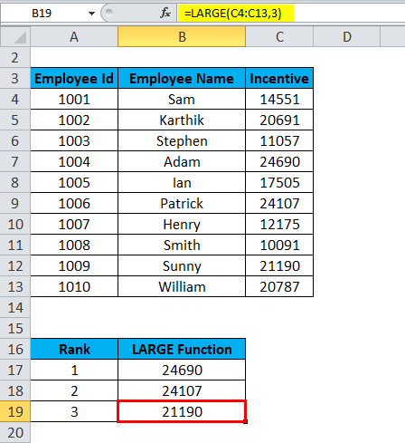
=LARGE(C4: C13,3)
The Result is:
The final results are:
Example #2
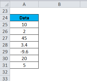
Let’s consider the below example with some values.
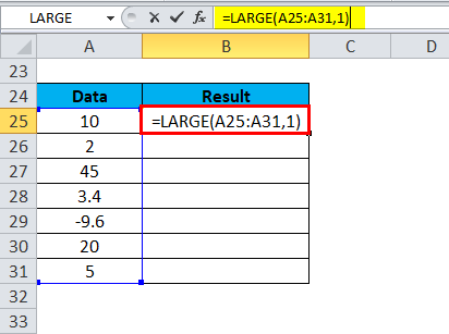
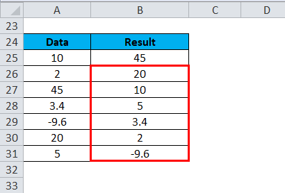
We need to arrange the above data in the order of Largest to smallest. With the help of the LARGE function, we can do this very easily.
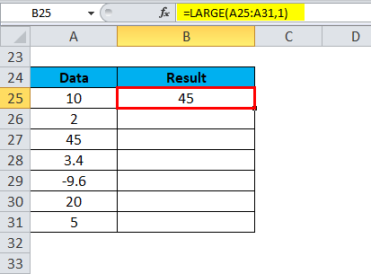
=LARGE(A25:A31,1)
The Result is:
Similarly, we find other values
Example #3
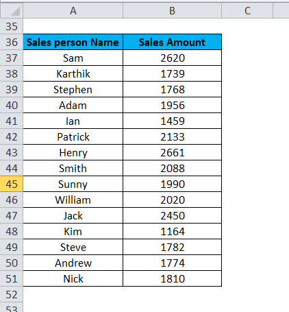
Let’s assume Sales data is given, and we want to see the total sales from the top 5 performers.
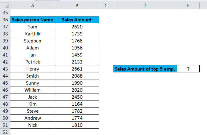
We want to see the sales done by the top 5 sales employee:
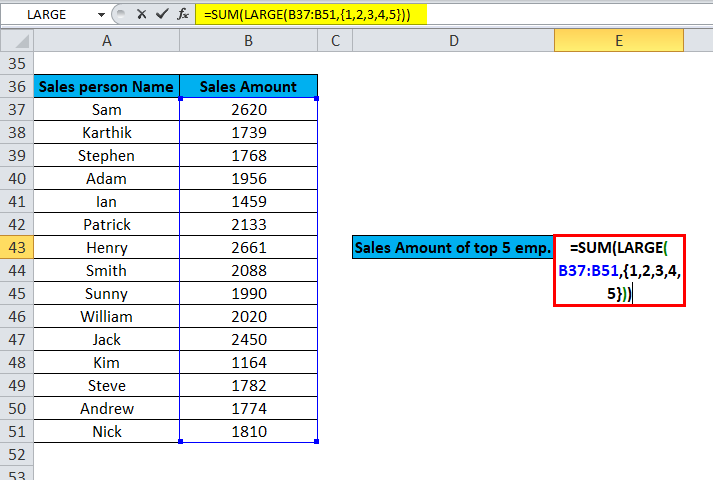
We will apply the LARGE function to select the top 5 sales performers by passing the positions from 1 to 5 as an array as a second argument (k) position and summing those values.
The formula used for solving this problem is:
=SUM (LARGE(B37:B51,{1,2,3,4,5}))
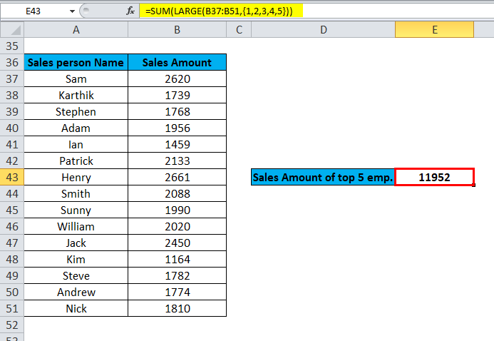
The final result is:
Things to Remember
- If the LARGE function returns the error value #NUM!, it means
- The second argument value (k) is less than 1 or greater than the number of values in the given array.
- The given array is empty.
- Suppose the function returns the error value #VALUE! – means the second argument (k) is non-numeric.
- The LARGE function is used to sort the data.
Recommended Article
This has been a guide to Excel LARGE Function. Here we discuss the LARGE Formula and how to use the LARGE function, along with practical examples and a downloadable Excel template. You can also go through our other suggested articles –
