ROUNDDOWN Function in Excel (Table of Contents)
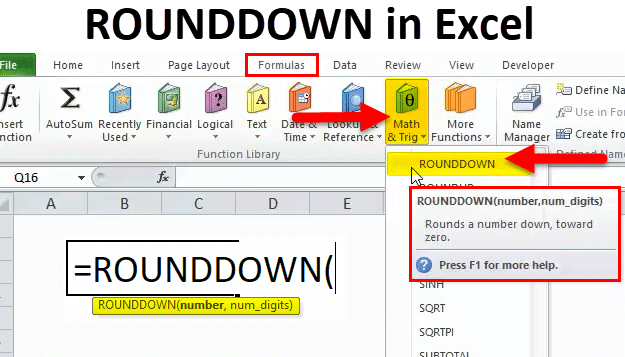
ROUNDDOWN in Excel
Rounddown function in excel rounds off the decimal number, but it also allows us to eliminate the complete digits after the selected number and replaces those numbers after decimal with Zeros. For example, if we have a number with 4 decimal digits and we select 2 in place of num_digit then after 2 digits of decimal we will be having 00 till the last decimal digit that number has.
ROUNDDOWN Formula in Excel:
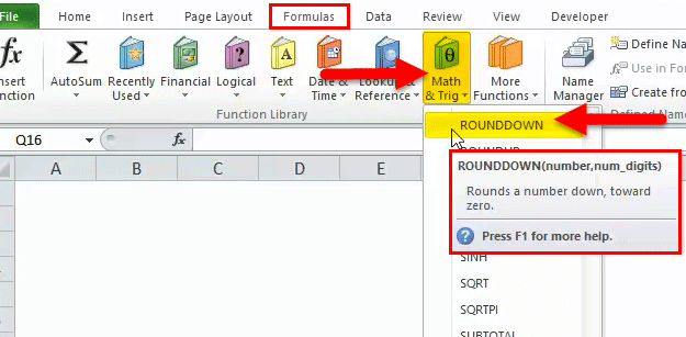
Below is the ROUNDDOWN Formula:
The ROUNDDOWN function syntax or formula has the below-mentioned arguments:
number: It is the number that you want to round down. It is a compulsory & required argument.
It can be entered as a cell reference, number, function or formula.
num_digits: It is the number of digits to which number should be rounded down
or
We have to specify how many units (decimal places) you want to round it to
Prior to applying the round down function, you should be aware of how to determine the number of digits? Suppose I have a number 950.134
9 5 0 . 1 3 4
| Hundreds | Tens | ones | Tenth | Hundredth | Thousandth |
Place value towards Left-hand side data is called as ones, tens & hundreds. Whereas place value after a decimal point, i.e. towards the right is called Tenth, Hundredth & Thousandth.
How to Use ROUNDDOWN Function in Excel?
ROUNDDOWN Function is very simple to use. Let us now see how to use the ROUNDDOWN function in Excel with the help of some examples.
Example #1
Round down a number to zero decimal place
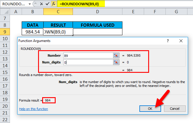
In the below-mentioned example, Cell “B9” contains a number with decimal values. i.e. 984.5395, With the help of the ROUNDDOWN function, I need to round down a number to zero decimal value in the cell “C9.”
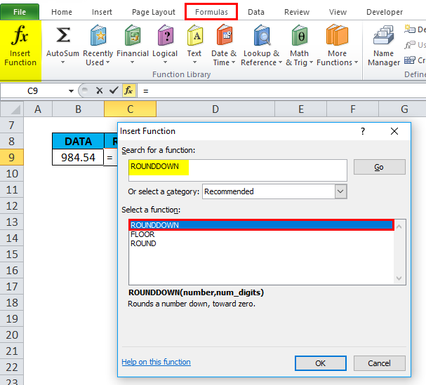
Let’s apply the ROUNDDOWN function in cell “C9”. Select the cell “C9” where the ROUNDDOWN function needs to be applied.
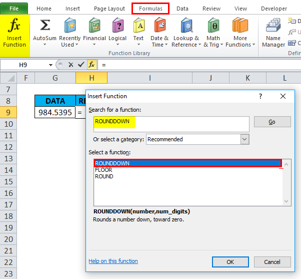
Click the insert function button (fx) under the formula toolbar, a dialog box will appear, type the keyword “ROUNDDOWN” in the search for a function box, a ROUNDDOWN function will appear in select a function box. Double click on a ROUNDDOWN function.
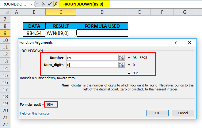
A dialog box appears where arguments for the ROUNDDOWN function needs to be filled or entered
, i.e. =ROUNDDOWN(number, num_digits)
number: It is the number that I want to round down. Here either 984.5395 or B9 cell reference is entered to get the desired output. Here I mentioned the reference cell, i.e. “B9.”
num_digits: I want the number with zero decimal value. I have to enter “0”, or it can be left blank. Note: by default, if we don’t enter any value. it takes zero
Click ok after entering both the arguments.
Here =ROUNDDOWN(B9,0) formula results in or Rounds 984.5395 down to a number with zero decimal value, i.e. 984
Example #2
Round down a number to two decimal places
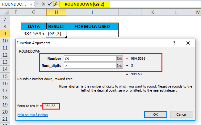
In the below-mentioned example, Cell “G9” contains a number with decimal values. i.e. 984.5395, With the help of the ROUNDDOWN function, I need to round down a number to two decimal value in the cell “H9.”
Let’s apply the ROUNDDOWN function in cell “H9”. Select the cell “H9” where a ROUNDDOWN function needs to be applied.
Click the insert function button (fx) under the formula toolbar, a dialog box will appear, type the keyword “ROUNDDOWN” in the search for a function box, a ROUNDDOWN function will appear in select a function box. Double click on a ROUNDDOWN function
A dialog box appears where arguments for the ROUNDDOWN function needs to be filled or entered
i.e. =ROUNDDOWN(number, num_digits)
number: It is the number that I want to round down. Here either 984.5395 or G9 cell reference is entered to get the desired output. Here I mentioned the reference cell i.e. “G9”
num_digits: I want the number with two decimal values. I have to enter “2”
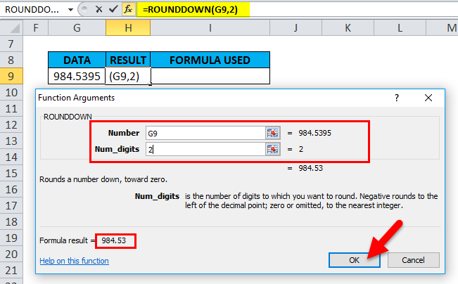
Click ok after entering both the arguments.
Here =ROUNDDOWN(G9,2) formula results in or Rounds 984.5395 down to a number with two decimal value, i.e. 984.53
Example #3
For a Negative value or Dataset
In the below-mentioned example, Cell “B16” contains a negative number with decimal values. i.e. -984.5395, With the help of the ROUNDDOWN function, I need to round down a number to the nearest integer in the cell “C16.”
Let’s apply the ROUNDDOWN function in cell “C16”. Select the cell “C16”. where a ROUNDDOWN function needs to be applied.
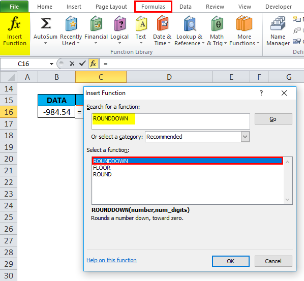
Click the insert function button (fx) under the formula toolbar, a dialog box will appear, type the keyword “ROUNDDOWN” in the search for a function box, a ROUNDDOWN function will appear in select a function box. Double click on a ROUNDDOWN function.
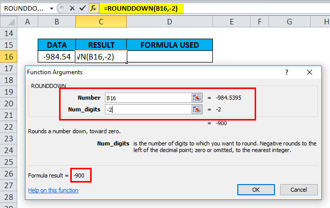
A dialog box appears where arguments for the ROUNDDOWN function needs to be filled or entered
, i.e. =ROUNDDOWN(number, num_digits)
number: It is the number that I want to round down. Here either -984.5395 or B16 cell reference is entered to get the desired output. Here I mentioned the reference cell, i.e. “B16.”
num_digits: I have to enter “-2” I want the number rounded down to the left side of the decimal point
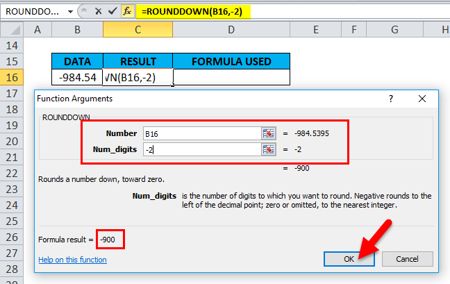
Click ok after entering both the arguments.
Here =ROUNDDOWN(B16,-2) formula results in or Remove all the decimals in -984.5395 and rounds integer down to the nearest hundred, i.e. -900
Things to Remember
A ROUNDDOWN function can round either to the right or left side of the decimal point.
- If the num_digits argument is greater than 0, Then it results in, or number is rounded down to the specified number of decimal places to the right of the decimal point.
E.G. =ROUNDDOWN(984.5395,2) returns the value 984.53
- If a num_digits argument is equal to 0, Then it results in, or number is rounded down to the nearest integer
E.G. =ROUNDDOWN(984.5395,0) returns the value 984
- If a num_digits argument is lesser than 0, Then it results in, or number is rounded down to the left side of the decimal point (i.e. to the nearest 10, 100, 1000, etc.).
E.G. =ROUNDDOWN(-984.5395,-2) returns the value -900
Recommended Articles
This has been a guide to Excel ROUNDDOWN function. Here we discuss the ROUNDDOWN Formula and how to use the ROUNDDOWN function in Excel, along with practical examples and a downloadable excel template. You can also go through our other suggested articles –
