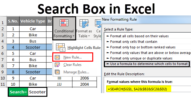
Search Box in Excel
Search Box in Excel is a customized feature that lets you easily locate and highlight specific data in a worksheet. It’s like searching for a book in a library. If you know the book’s title, you can search for it in the catalog instead of searching through every book on the shelves.
Similarly, the Search Box lets you quickly locate specific words or numbers in a large dataset. It helps you find what you need without manually searching through everything.
Search Box in Excel Syntax
where:
- search_text (required argument): This is the text or substring you want to search for within the larger text string.
- within_text (required argument): This is the text string to search for the search_text.
- start_num (optional argument): This is the starting position from which you want to begin the search. If omitted, Excel assumes it to be 1 (the beginning of the text string).
Please remember that the SEARCH function in Excel is case-insensitive, which means it will not distinguish between uppercase and lowercase letters. If a case-sensitive search is necessary, use the FIND function, which has a similar syntax but is case-sensitive.
How to Create a Search Box in Excel?
To create a search box in Excel,
Step 1: Go to the Conditional Formatting option under the Home menu ribbon.
Step 2: Select “New Rule” from the drop-down menu. This creates a new formatting rule using a formula.
Step 3: The rule box will appear. Use the SEARCH function therein to specify the text you want to search for.
Step 4: Enter the text you want to find in the “Find Text” option.
Step 5: Choose the formatting options, such as cell or font color, for the cells containing the search results.
It will highlight those value cells with the selected color within the selected text range.
Now, let’s use some examples to understand how to create your own Search Box in Excel.
Examples of Search Box in Excel
Example #1
Consider that you have the data of a company that sells and purchases used vehicles. However, the enormous amount of data makes searching for a particular car model name difficult. To simplify this process, you want to create a search box in Excel that highlights all values related to “Scooter” instead of manually searching through every cell.
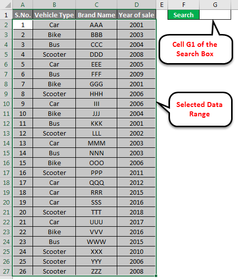
Here’s a screenshot to illustrate what your data looks like.

Solution:
1. Open an Excel worksheet and go to the cell where you wish to create the search box. Here, we have selected G1 as the search box cell. You can highlight the selected cell to distinguish it from other cells.
2. Select the entire data range from where you want the data, or the value searched. The selected range, in this case, is A2: D27 (as shown below).
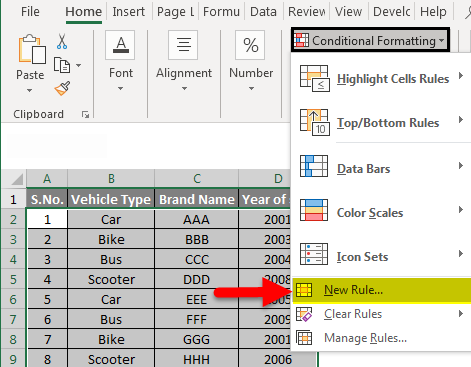
3. Once you have selected the entire data range, go to Conditional Formatting and select New Rule.
4. On the next window, click the option. Use a formula to determine which cells to format.

After this, enter the following formula below the text box.
=SEARCH($G$1,$A2&$B2&$C2&$D2)
The formula used above is deciphered after the last step for this example.
5. After writing the above formula in the space provided, click the Format button below it to select the color in which the searched (and matched) values will be highlighted.
This can be possible by selecting the Fill button on the next window and selecting the color.

6. After this, click OK, and you will see that all the fields in your sheet are now highlighted with the selected color, as shown below:
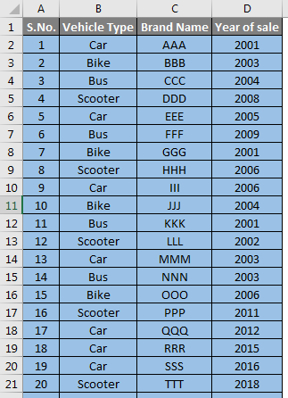
7. Now, you can search for the desired keyword and see that all the rows containing that keyword are now highlighted with the selected color.
For example, let’s try searching for the item named Scooter. You’ll see that all the rows with the word scooter have been highlighted.
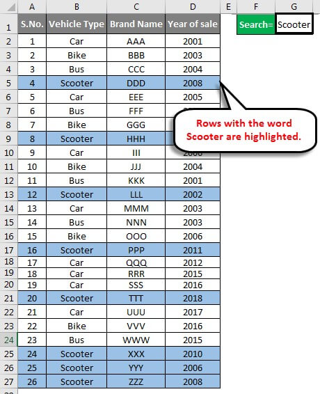
This simplifies the process of looking for any value. For example, after highlighting the fields related to Scooter, we can further refine our search results by applying a filter based on the color of those highlighted fields.
Now let’s understand the meaning of the parameters used in the Search formula and how it worked for us in Excel.
Explanation of Formula
Let us now try to understand what each parameter within the formula of Search means in Excel. Consider the formula that we used.
=SEARCH($G$1, $A2&$B2&$C2&$D2)
Let’s have a look at each parameter individually.
1. $G$1
=SEARCH($G$1, $A2&$B2&$C2&$D2)
This parameter defines the location where we wish to apply the search rule. We can either type the cell number manually or select the cell by clicking on it (after writing =SEARCH) in the conditional formatting rule window.
2. $A2&
=SEARCH($G$9,$A2&$B2&$C2&$D2)
In the parameter “$A2&” of the formula, “A” indicates the column in the data source, and “2” indicates the starting row for the search. So, ‘A2’ means we wish to search for the data in column ‘A’ starting from the 2nd row. Adding a “$” before “A” locks the column reference, so it won’t change when we copy the formula. Thus, the search location will remain fixed even if we change the location of the search box.
The “&” symbol is useful for joining or connecting text in different cells. In this formula, combining the values in cells A2, B2, C2, and D2 into a single string is useful.
$A2&$B2&$C2&$D2.
This is the text string within which we want to search for the value specified in G9. The “&” symbol will join or concatenate the values in cells A2, B2, C2, and D2 into one string.
Now, let’s say we want to find the brand names of scooters sold in the year 2008.
To do this, we can apply a filter in the “Year of Sale” field.
Let us have a look at the screenshot attached below.
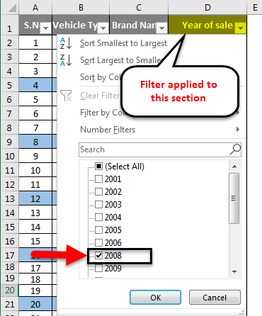
We get the following result once we apply the filter and click OK. There are 2 brands whose scooters made sales in 2008, as shown below.

This is how it can help simplify the search process.
We can even use filters to perform a search as we did above, but then we would need to apply multiple filters to look for multiple things. Moreover, the example that we saw here had limited data. There may be cases when the amount of data in a sheet is huge. A Search Box can help us in all such situations as it creates a search criterion for the entire sheet.
Example #2
Using Search Box with Filter Function in Excel
To create a search box in Excel, use the FILTER function (here, we are not applying a filter), an easy and efficient way to filter data based on criteria. Here are the steps to create a search box in Excel using the FILTER function, along with the following illustration for better understanding:
In the below screenshot, we compare the data for sales made by different sales executives in every region and create a separate search box to search and filter data from the original data. We want to determine sales done by a particular sales executive or a region and the quantum of sales generated using the search box and filter function together.
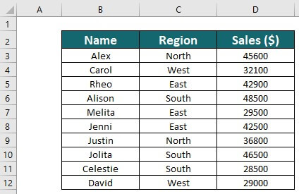
Solution:
Step 1: Choose a cell where you want to create the search box. For example, you can select cell G2 in the worksheet.
Step 2: Create a result box where you want the search results displayed. For example, create a result box from F5 to H6. Here, separate columns for original data are useful to search in that column.
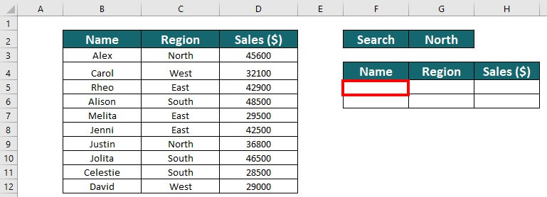
Step 3: In cell F5, enter the following filter formula: =FILTER(B3:D12, C3:C12=G2, “NO MATCH FOUND”)
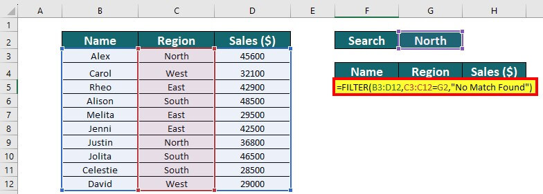
Here’s the role of each part of the formula:
- B3:D12: This is the range of values that you want to filter.
- C3:C12=G2: This is the criteria that you want to use for filtering. Adjust it based on your specific criteria. This example compares the values in the range C3:C12 with the value in cell G2 (the value entered in the search box).
- “NO MATCH FOUND”: This value will get displayed in the result box if no entries meet the filtering criteria. You can customize it to your preference.
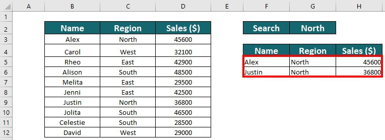
Step 4: Start Using the Search Box once you have entered the FILTER formula. Enter a name or other search criteria in the search box (cell G2 in this example), and you will see the filtered results in the result box (cells B3 to D12). Here, since we have searched for the North region in filter results, Alex and Justin as shown under names as they are from the North region. Their sales figures as given accordingly.
You can also try this for other regions like the East.
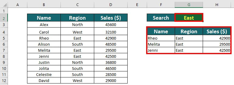
With the FILTER function, you can easily create a search box in Excel that dynamically filters data based on your criteria, making it a powerful tool for data analysis and manipulation.
Things to Remember
- Make sure that you enter the formula correctly in the conditional formatting window.
- Use the $ sign as shown in Example 1 to ensure no deviation.
- The & sign is useful for adding more columns in the formula. Ensure not to put the & sign at the end of the formula.
- Though both Search Box and Filters are useful for fetching outputs based on various conditions, we should not use them interchangeably as they solve unique purposes in different manners. This box can also be useful to enhance the function of a filter.
Frequently Asked Questions (FAQs)
Q1. Where is the search bar on Excel?
Answer: In Microsoft Excel, the search bar is the “Find” tool, and it is typically found in “Editing” on the “Home” tab. It is a binoculars icon labeled “Find & Select.” To get to it, open Excel, go to the “Home” tab, find the “Editing” group, and then click the “Find” tool. This will open a search bar or dialogue box in which you can enter the text or value searched for within the Excel worksheet.
Q2. Why is my search box not working in Excel?
Answer: There could be many reasons why the Microsoft Excel search box or “Find” tool isn’t working. Some possible explanations and solutions are as follows:
- No text or value to search: Check that you have entered the correct search text or value in the search box’s “Find what” Excel may be unable to find matches if the search text is blank or contains a typo.
- Active cell outside the search range: Excel looks for text or values within the current worksheet or range. Make certain that the active cell is within the search range. Excel may be unable to find matches if the active cell is outside the search range.
- Incorrect search options: Excel’s “Find” tool provides several search options, including match case, search direction, and search by rows or columns. Check that you’ve selected the appropriate options based on your search criteria. Excel may be unable to find matches if the search options are not properly configured.
- Protected worksheet: If the worksheet or workbook is password-protected or has restricted permissions, the “Find” tool may not function as expected. In such cases, you may need to unprotect the worksheet or workbook before using the “Find”
- Excel version or installation issues: Excel version or installation issues: In some cases, problems with Excel itself, such as software bugs or installation errors, can interfere with the “Find” tool’s functionality. In such situations, you may need to update or reinstall Excel or contact Microsoft or your IT department for assistance.
Suppose you’ve checked all the above options, and the search box still doesn’t work in Excel. In that case, it’s best to consult the Excel document or Help feature or contact Microsoft support or your IT department for further troubleshooting and resolution.
Q3. What are the functions of a search bar?
Answer: A search bar is a tool that allows users to find specific content within a dataset. It has filtering capabilities auto-suggestion feature and can function as a navigation tool. It may also provide error handling, a history, and personalized recommendations. Finally, search results are visible for users to browse and select from.
Recommended Articles
This has been a guide to Search Box in Excel. Here we discuss How to Create a Search Box in Excel and the Usage of a Search Box in Excel, along with practical examples and a downloadable Excel template. You can also go through our other suggested articles –

