Updated July 5, 2023
Introduction to Excel SUM MAX MIN AVERAGE Functions
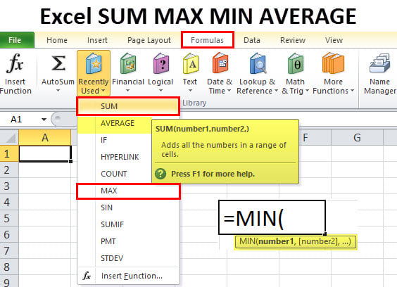
Excel can be overwhelming for beginners, but with a little practice, you can use it like a pro! A good starting point would be to learn some of Excel’s basic functions. By learning the most commonly used functions, such as SUM, MAX, MIN, and AVERAGE, you can efficiently perform calculations over a range of values within a worksheet.
These Excel SUM MAX MIN AVERAGE functions can come in handy for all sorts of tasks. For instance, you can use the SUM function to add sales figures quickly. The MAX and MIN functions can help you find the highest and lowest employee salaries for a department. The AVERAGE function can be helpful if you are trying to determine the average grades of students or the average sales of a company.
To help you get started, we’ll walk you through each function of the Excel SUM MAX MIN AVERAGE functions with multiple examples.
1. SUM Function in Excel
The SUM is a mathematical function that adds up a range of values. One can use the SUM function to quickly find the total of a set of values, such as company expenses, sales figures, or test scores.
The Syntax of the SUM function is:
The function takes the following arguments :
number1: It indicates the first numerical value we want to add.
number2: It marks the second numerical value we want to add.
It takes a maximum of 255 arguments, and they can be numbers, cell references, cell ranges, constants, arrays, and the results of other formulas or functions.
How to Use SUM Function in Excel?
Example 1
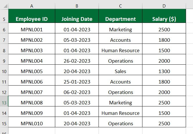
We want to find the total salary of employees working in different company divisions using the SUM function in Excel.
Solution:
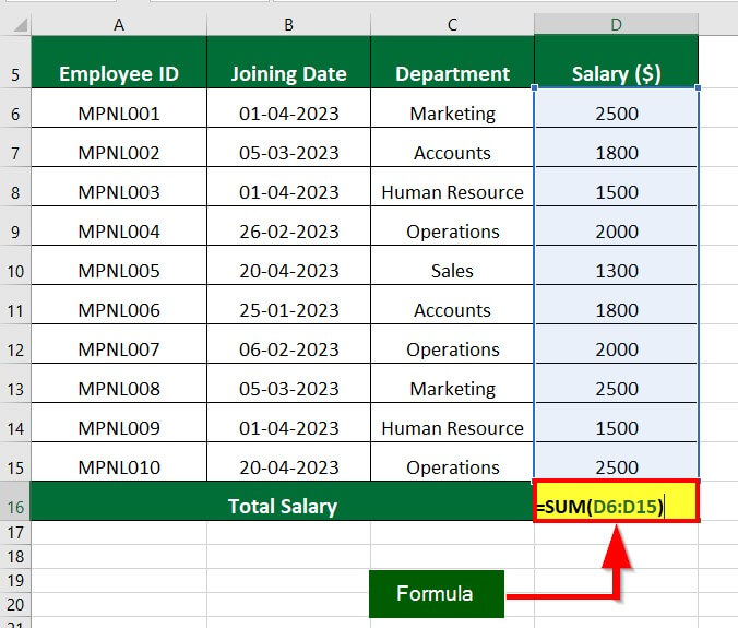
Step 1: In an empty cell (Cell D16), enter the formula =SUM(D6:D15).
The formula adds all the values between the range D6:D15.
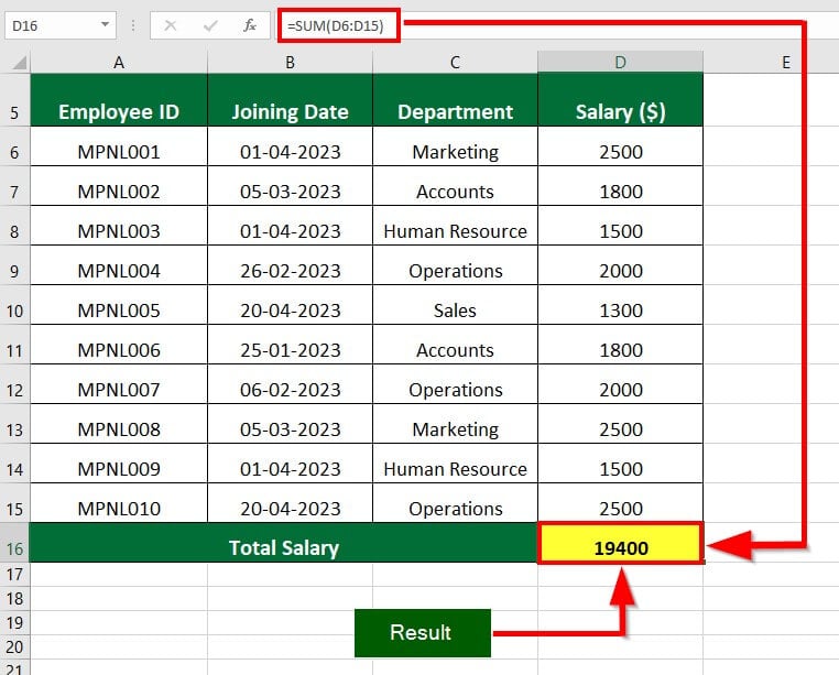
Step 2: Press Enter key to obtain the result, which is 19400.
Example 2
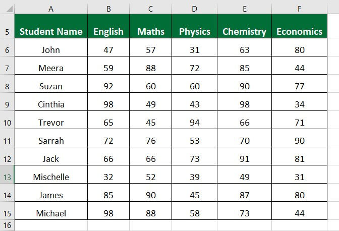
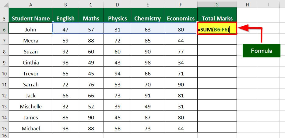
Suppose we have the test scores of 10 students in English, Maths, Physics, Chemistry, and Economics. We want to determine the total marks of each student.
Solution:
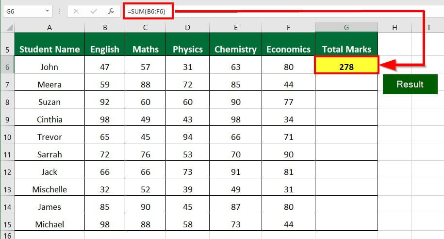
Step 1: Create a new column heading Total Marks and enter the formula =SUM(B6:F6) in cell G6.
The formula adds all the values (in this case, marks of John in each subject) and gives the output of 278.
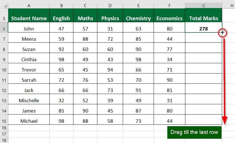
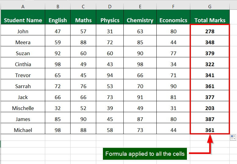
Step 2: Drag the formula in the remaining cells to find the total marks of all students.
The image below illustrates the total marks that each student has scored.
2. MAX Function
MAX is a mathematical function determining the largest value in a given cell- range. You can use the function to find the highest monthly sales figure, test score, or temperature in a given period.
Syntax:
The MAX function in Excel accepts the following arguments:
number1- It represents the first integer we want to compare
number2-It represents the second integer we want to compare
In Excel 2007 and newer versions, the MAX function can handle a maximum of 255 arguments. However, for Excel 2003 and older versions, the MAX function can only process up to 30 arguments.
How to Use MAX Function?
Example 1
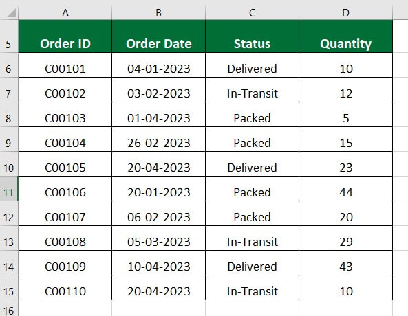
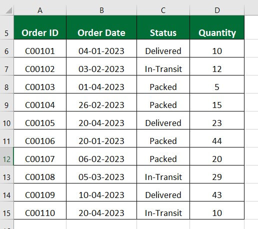
A courier company has 10 orders and wants to determine the maximum quantity in an order using the MAX function in Excel.
Solution:
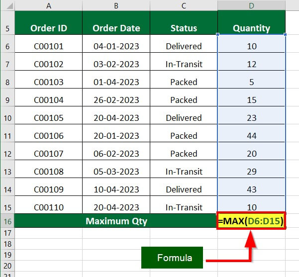
Step 1: In a empty cell (Cell D16), enter the formula =MAX(D6:D15)
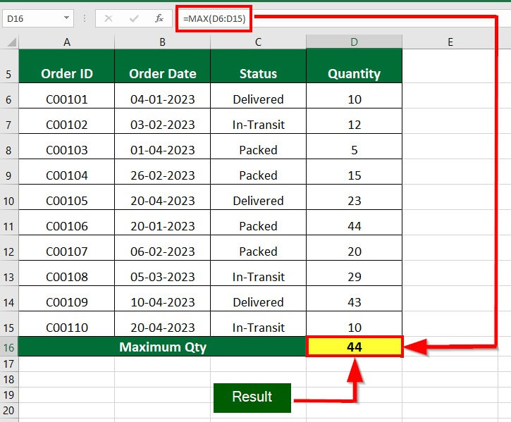
The formula finds the integer holding the largest value between the range D6:D15.
Step 2: Press Enter to see the result.
Example 2
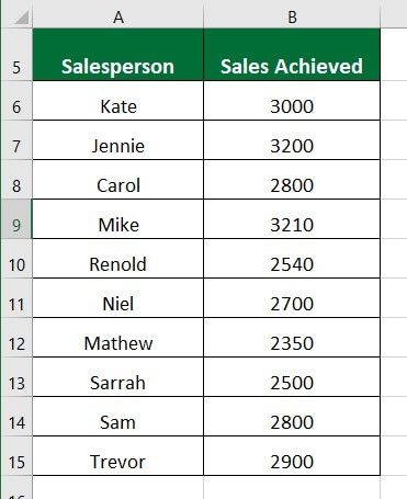
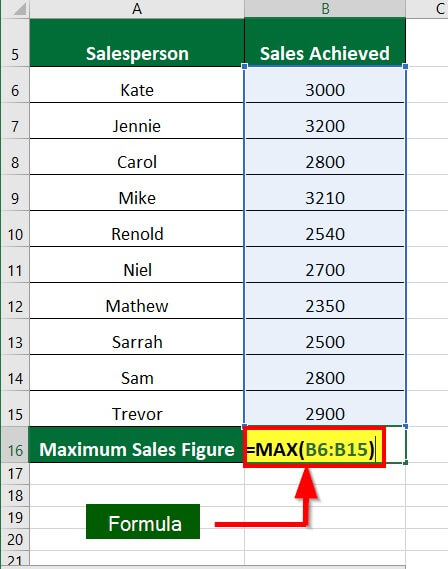
You want to find out the highest sales record achieved by the sales representatives in your organization to acknowledge their achievement with a prize or recognition.
Solution:
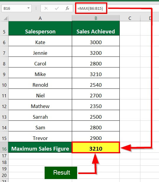
Step 1: In an empty cell (Cell B16), enter the formula =MAX(B6:B15).
The formula determines the number with the highest value within B6 to B15.
Step 2: Press Enter key to get the result
3. MIN Function
The Excel MIN function provides the smallest value within a range and is particularly useful in data analysis and decision-making. For instance, finance professionals may use it to identify the lowest price point for a product over a given period.
Syntax:
The MIN function in Excel takes the following arguments:
number1- It represents the first integer we want to compare
number2-It represents the second integer we want to compare
The MIN function in Excel can support up to 255 arguments in Excel 2007 and later versions. In 2003 and earlier versions of Excel, it can only accept up to 30 arguments.
How to Use the MIN Function?
Example 1
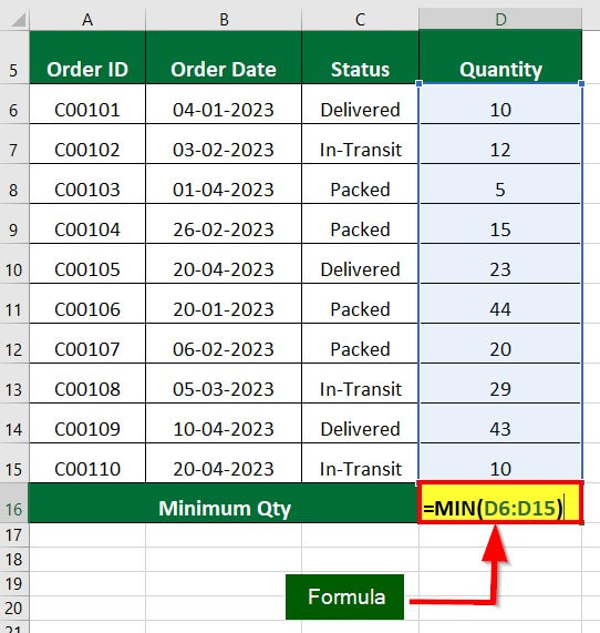
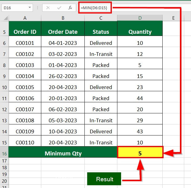
A courier company has 10 orders and intends to find the minimum quantity of items within an order using the MIN function.
Solution:
Step 1: In a empty cell (Cell D16), enter the formula =MIN(D6:D15)
The formula finds the integer holding the smallest value between the range D6:D15.
Step 2: Press Enter key to get the result.
Example 2
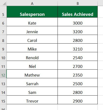
You want to find out the lowest sales a salesperson in your company has achieved using the MIN function.
Solution:
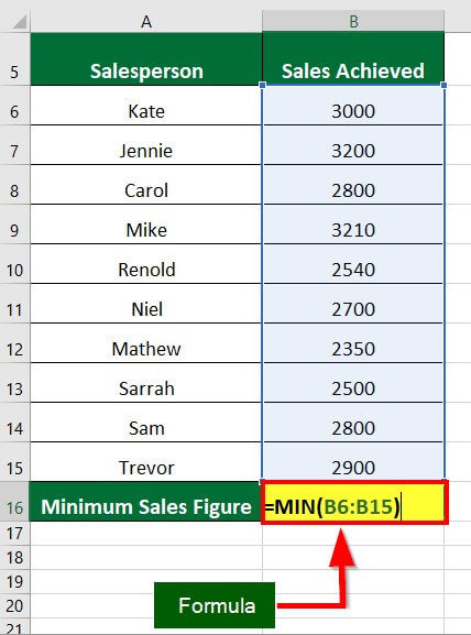
Step 1: In an empty cell (Cell B16), enter the formula =MIN(B6:B15).
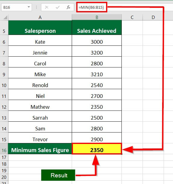
The formula determines the number with the lowest value within B6 to B15.
Step 2: Press Enter.
4. AVERAGE Function in Excel
In Excel, the AVERAGE function determines the arithmetic mean of a range of values. The function takes a series of numbers and returns the sum divided by the count of those numbers. It helps users find a company’s average monthly, quarterly, or yearly revenue or expenses. Students can use it to calculate their average grade across multiple subjects.
Syntax
The AVERAGE function takes the following arguments
Number 1 indicates the first number or range of numbers we want to take an average of.
Number 2 is an optional argument representing a second number or range of numbers we want to find average.
The function allows up to 255 arguments and ignores text or blank cells.
How to Use the AVERAGE Function?
Example 1
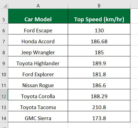
A car manufacturer wants to determine the average speed of its various models by using the AVERAGE function in Excel.
Solution:
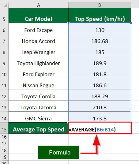
Step 1: In an empty cell (Cell B15), enter the formula =AVERAGE(B6:B14)
The formula calculates the average of all the values (here, speed) in the range B6:B14.
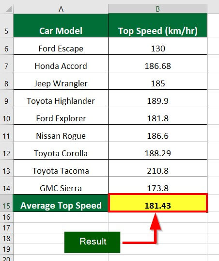
Step 2: To see the result, press the Enter key.
Example 2
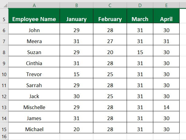
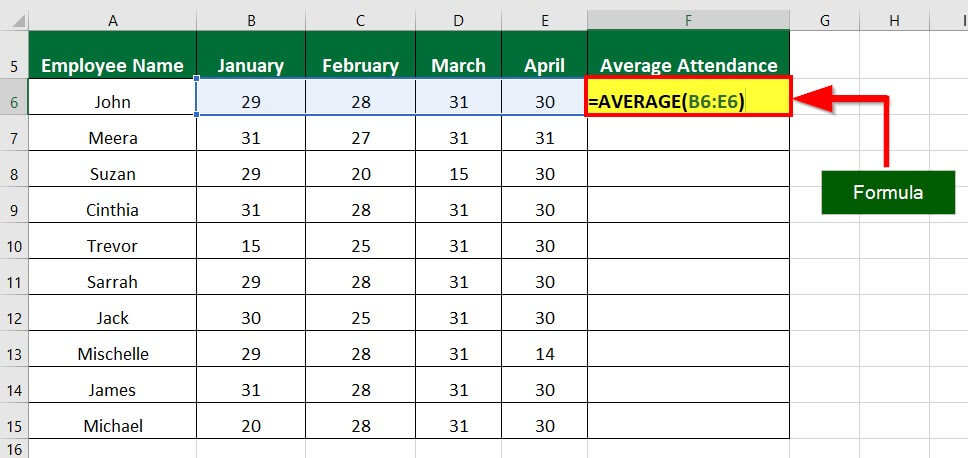
An organization’s HR department aims to determine its employees’ average attendance for January, February, March, and April using the AVERAGE function in Excel.
Solution:
Step 1: Create a new column (F) with the heading “Average Attendance” and enter the formula =AVERAGE(B6:E6) in cell F6.
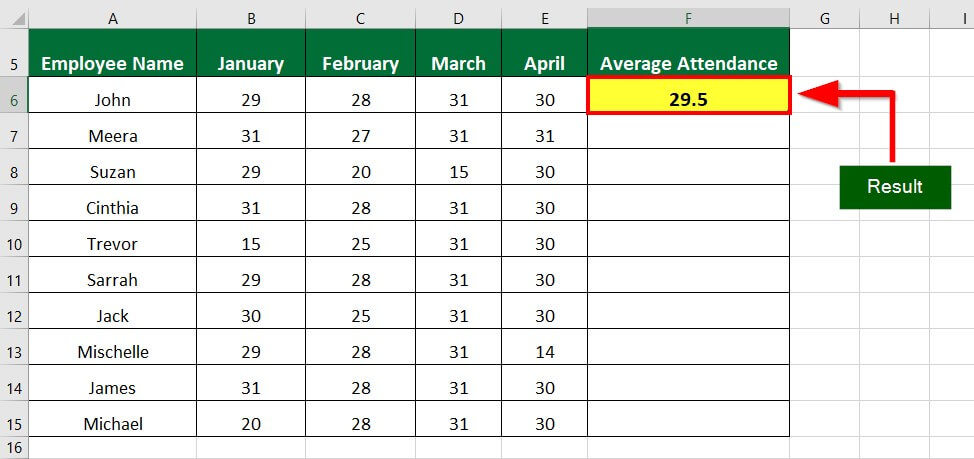
The formula calculates the average of all the values (here, no. of days John was present) in the range B6:E6.
Step 2: Press Enter key to obtain the result
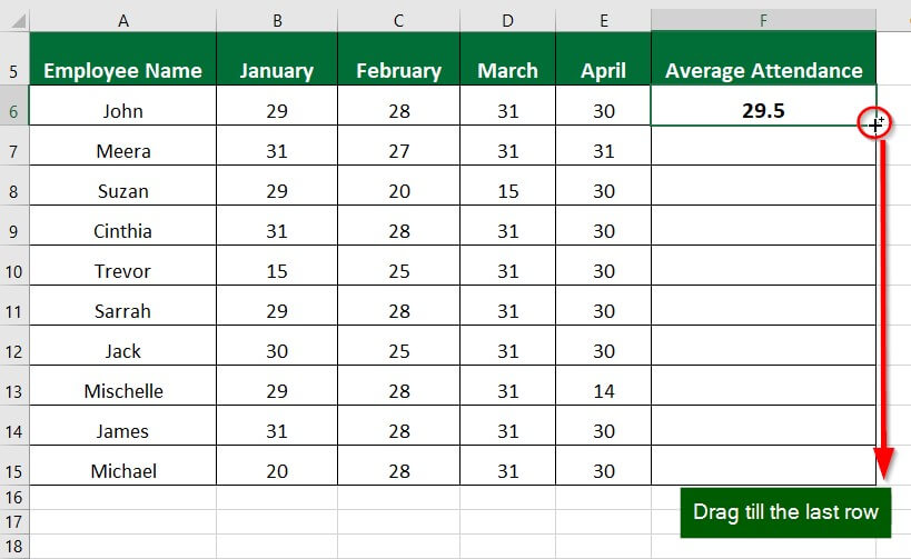
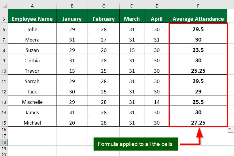
Step 3: Drag the formula in the remaining cells to get the average attendance for all the employees.
The below image illustrates the average attendance of all the employees.
Frequently Asked Questions (FAQs)
Q1. How do you write an average function in Google Sheets?
Answer: To write an average function in Google Sheets, follow these steps:
Step 1: In the desired cell, write the formula =AVERAGE(range of cells)
Step 2: Press Enter.
Alternatively,
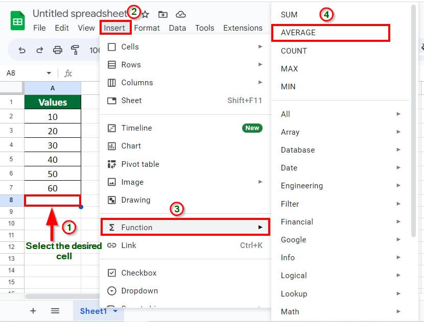
Select the desired cell & Go to Insert > Function > Average.
It inserts the average function into the active cell, where we must select the range of values to calculate the average.
Q2. What is the shortcut to SUM in Excel?
Answer: In Excel, the shortcut to calculate the sum of a range of cells is to press the keys “ALT” and “=” together. This key combination automatically inserts the SUM function into the active cell and selects the range of cells containing the values. The user can then press “Enter” to display the result.
Q3. How do I get the max and min date in Excel?
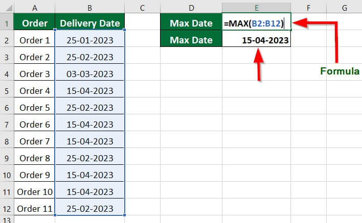
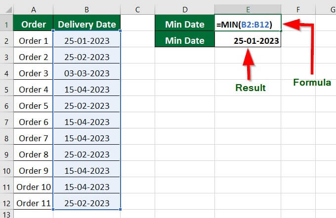
Answer: Excel stores dates as whole numbers; therefore, we can utilize the Excel MAX function to find the latest date and the MIN function to get the earliest date in a given range of dates.
To get the MAX(latest) date, follow these steps:
Step 1: In an empty cell, enter the formula =MAX(B2:B12)
Step 2: Press Enter to get the result as shown in the image below
To get the MIN (earliest) date, follow these steps:
Step 1: In an empty cell, enter the formula =MIN(B2:B12)
Step 2: Press Enter to get the result as shown in the image below
Q4. How do you find the minimum value in Excel with multiple criteria?
Answer: To find the minimum value in Excel on the basis of multiple criteria, you can use the MIN and IF functions together.
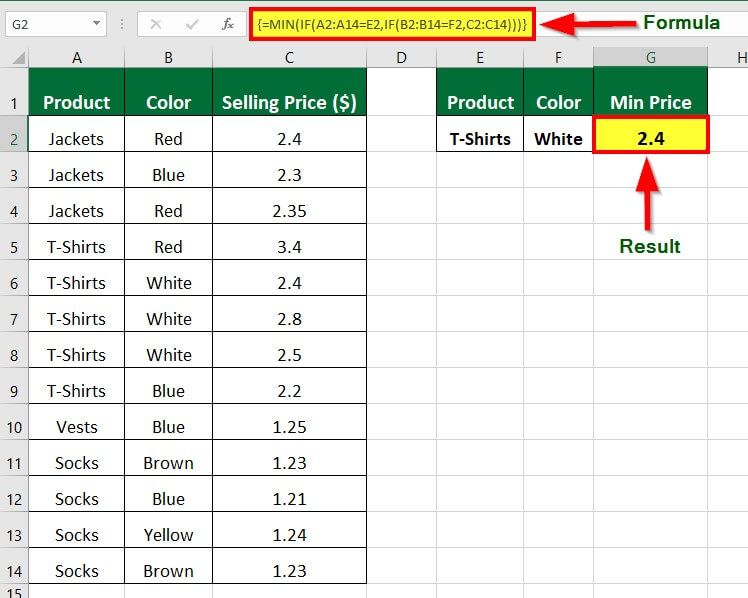
For instance, if you want to calculate the minimum selling price of a white color T-shirt, the below-given steps will help you learn how this method works.
Step 1: In an empty cell, enter the formula =MIN(IF(A2:A14=E2,IF(B2:B14=F2,C2:C14)))
Step 2: Press Enter key to get the result
Explanation:
- The first IF function compares the cells in the range A2 to A14 (containing product names) to the value in cell E2 (which has “T-shirt”).
- If a cell in the range matches, the second IF function compares the corresponding cell in the range B2 to B14 (which has colors) to the value in cell F2 (which has “white”).
- If the second comparison is also true, it passes the information to the MIN function, which determines the lowest value in the resulting price list and gives the minimum selling price of a white T-shirt.
Q5. Does the Excel average ignore blank cells?
Answer: Yes, the AVERAGE function in Excel only considers numbers ignoring blank cells, text values, and logical values.
Recommended Articles
The above article is a summary of Excel SUM MAX MIN AVERAGE Functions. Here we have discussed calculating Excel SUM MAX MIN AVERAGE functions with examples and a downloadable template. To learn more, please read the recommended articles,
