Updated May 8, 2023
SUMIF with OR (Table of Contents)
SUMIF with OR Function in Excel
SUMIF is a function that is very useful for finding the totals of similar values. It reduces the time when we are working with a large amount of data and need to calculate the sum of values of similar nature data. SUMIF is a combination of SUM and IF functions. SUMIF function will perform SUM(addition) when the IF condition is satisfied. It is very easy to apply.
Syntax of the SUMIF function
- Range – A range of cells on which the criteria or condition is applied. The range can also include a number, cell references, and names.
- Criteria – The condition in the form of a number, expression, or text defines which cells will be added.
- Sum_range – These are actual cells to sum. If omitted, cells specified in a range are used.
How to Use SUMIF with OR Criteria in Excel?
Using some examples, let’s understand how to use SUMIF with OR Function in Excel.
SUMIF with OR – Example #1
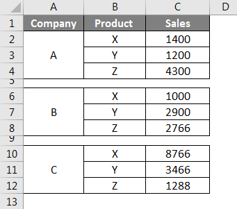
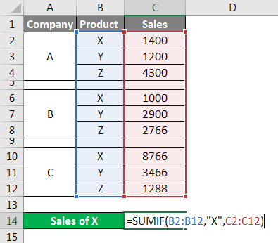
Consider a table having the sales data of companies A, B, and C for products X, Y, and Z.
In the above screenshot, we can observe the sales of products X, Y, and Z. Now, we need to calculate the sum of X sales in all three companies, A, B, and C.
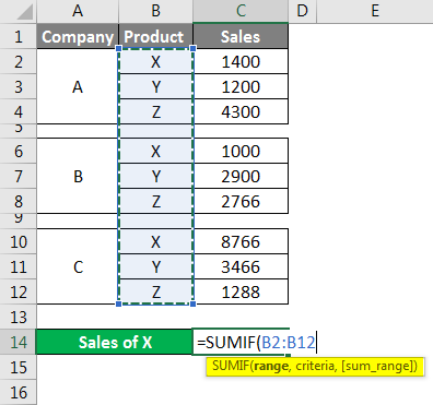
First, select a cell where we want the sum of ‘X’ sales results, then apply the function and select the range.
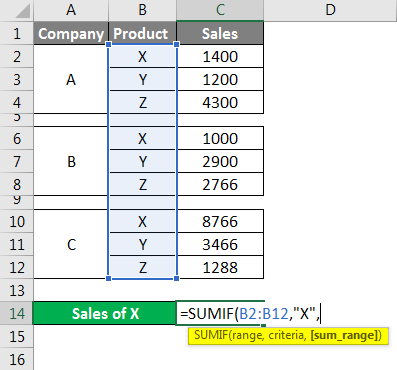
Here the range is from B2 to B12, so select that range then the function will automatically pick B2:B12, as shown in the above screenshot. Once the range is picked, give the comma as per syntax. Later give the “Criteria” here. Criteria are “X” as we want to find the SUM of X product sales, so give X and again comma.
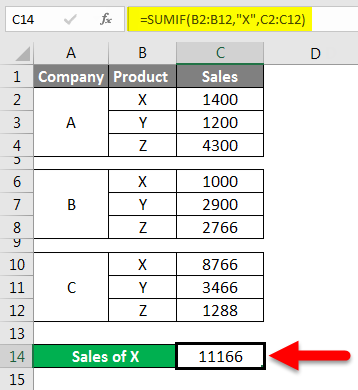
Last, we need to select the sum_range; here, sales is the range we need to add whenever the product is X; hence, select the sales range from C2:C12, as shown in the screenshot below.
The sum of sales of X across all three companies is 11166.
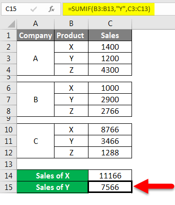
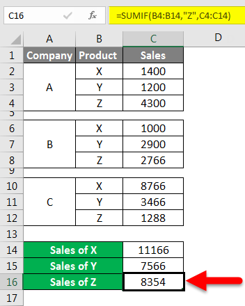
Similarly, we can find the sales of Y and Z also.
Use commas and a double column for criteria; otherwise, the formula will throw an error. Normally SUMIF will work on the logic, AND hence that is the reason where ever the criteria match, it will perform the addition and return the results.
Using normal SUMIF, we can perform SUM operation for only one criterion. If we use OR logic, we can perform SUM calculation for dual criteria.
For using OR logic, we should use SUMIFS instead of SUMIF because SUMIF can perform with single criteria, but SUMIFS can perform on multiple criteria as per our requirement.
SUMIF with OR – Example #2
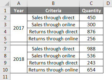
We will now consider a small table with data on sales and revenue online and direct as below.
Our task is calculating the total sales value, whether direct or online. Now we will apply the SUMIFS formula to find the total sales.
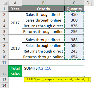
It is a bit different from the SUMIF as in this first, we will select the sum range. Here sum range means the column where the values are available to perform addition or sum.
Observe the above screenshot; the quantity is the column we need to add; hence select the cells from C2 to C10 as sum_range. The next step is the selection of criteria_range1.
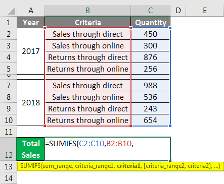
Here Criteria are “Sales through direct” and “Sales through online”; hence we need to select the column B data from B2 to B10.
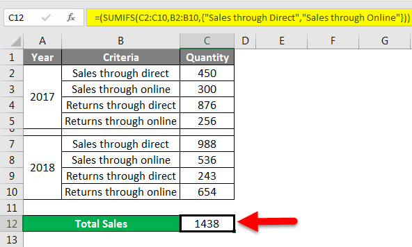
Later we need to give Criteria 1 and then Criteria _range2, criteria 2, but here we will make a small change. We will give criteria 1 and criteria 2 in a curly bracket like an array.
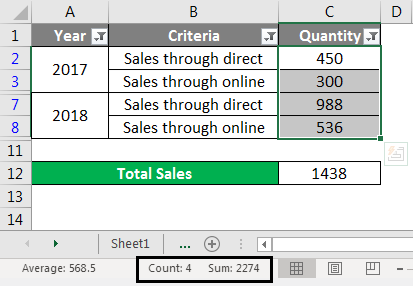
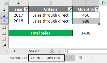
‘Apply a filter and filter only direct and online sales, select the entire quantity, and observe the total at the bottom of the screen. See, we got the result as 1438; let’s check whether it picked the total correctly or not. Observe the below screenshot; I have highlighted the count and sum of the values.
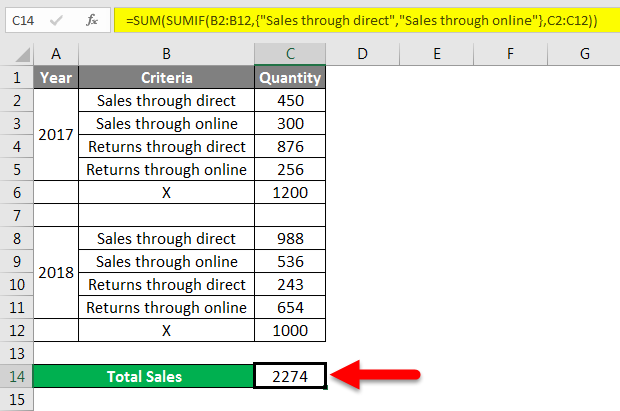
So, the total should be 2274, but we got the result of 1438. Then how this 1438 come, and what sum is this
Observe the above screenshot that 1438 is the total sales for sales through direct. The formula did not pick the sales online because we gave the formula in a different format, like an array. Hence, if we add one more SUM formula to SUMIFS, it will perform both criteria.
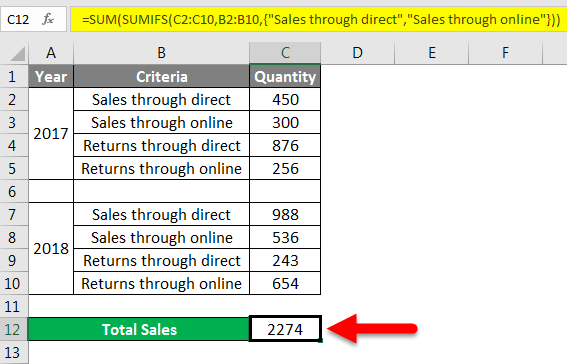
Observe the formula in the above screenshot one more SUM is added to the SUMIF, and the result is 2274.
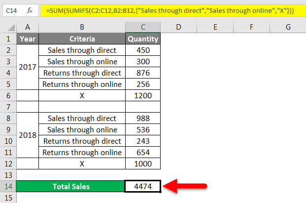
I will explain why we used another SUM function and how it works. When we give SUMIFS function with two criteria as an array, it will calculate the sum of sales directly and online separately. We have used another SUM function to add the sum of two sales to get the sum of both. If we want to add one more criterion, we can add it to the same formula.
Observe the formula; we added the criteria X in the curly brackets of an array, adding the quantity X to the existing sum quantity.
If you want to use only SUMIF and do not want to use SUMIFS, then apply the formula below.
Observe the formula in the above screenshot. In this case, first, we gave the criteria range, then criteria1 and criteria2, and the last sum_range.
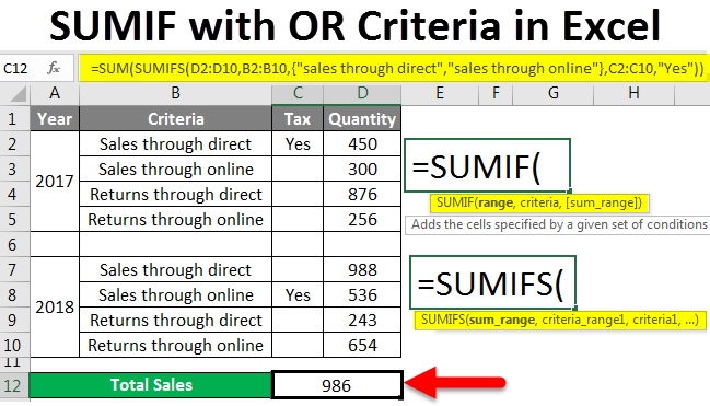
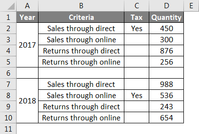
If we want to perform a sum based on two columns of data, consider the same data we used up to now. We need to add one more column, “Tax”, as below. There is a comment ‘yes’ under the TAX column.
Now the task is to calculate the sum of quantity for the sales director and sales online, which has “Yes” under the tax column.
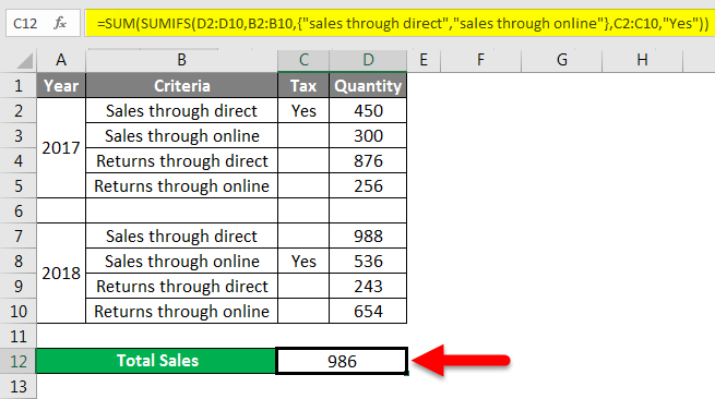
Apply the formula shown in the screenshot below to get the sum of sales with “Yes” under the Tax column.
After the normal SUMIFS formula, add another criterion range: tax column range C2 to C10, and give criteria “Yes” in double quotes.
Now the formula will check for criteria 1 with yes and criteria 2 with yes and add both.
Things to Remember About SUMIF with OR
- SUMIF follows the AND logic, meaning it will perform an addition operation if the criteria match.
- SUMIFS will follow the OR and logic so that we can perform multiple criteria at a time.
Recommended Articles
This is a guide to SUMIF with OR in Excel. Here we discuss how to use SUMIF with OR Criteria in Excel, practical examples, and a downloadable Excel template. You can also go through our other suggested articles–
