Updated June 3, 2023
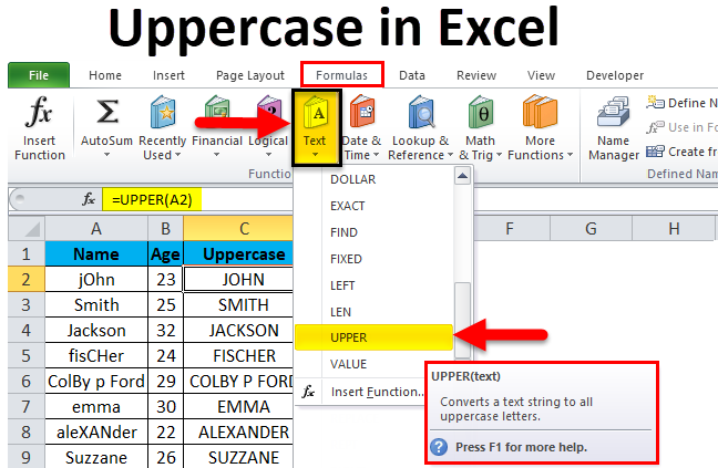
Introduction to Uppercase in Excel
The uppercase function in Excel converts any text into the uppercase format. This means we can have text which has all the letters in Caps. To apply Uppercase in Excel, type the equal sign in any cell and select the function UPPER. As per syntax, we will be selecting the only cell, the cell which contains only Text. We will see if it will convert the selected text into Uppercase.
Note: There is another formula for changing the case of words, like ‘PROPER’; however, we will discuss only ‘UPPER’ in this article as ‘PROPER’ changes only the first alphabet of a word.
Examples of Uppercase in Excel
Before learning how to change the words from lowercase to uppercase, let us look at how the upper function would work and what the output will look like.
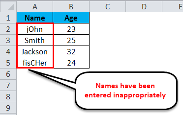
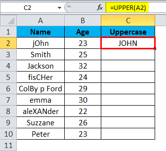
Consider the image given below that shows the names of various persons. You can see that the names have been entered inappropriately. Some alphabets are in lower case; some are in upper case.
This issue can be corrected, and we can convert the entire text into uppercase alphabets using a simple formula known as ‘Uppercase’.
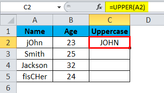
The formula that we used to get this conversion looks like this:
=upper (A2)
Similarly, we can convert other values.
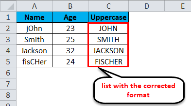
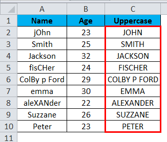
The image given below shows the list with the corrected format.
Explanation of Uppercase in Excel
As we have already discussed, unlike MS Word, MS Excel does not have an easy option of changing the case of words from lowercase to uppercase, so we use the formula of Uppercase. The only drawback of Uppercase is that we do not choose whether to change the case of all the letters or only the first letter. It always changes the case of all the alphabets present in a particular cell. Let us understand how to use this formula and what parameters to put in it.
The format to write this formula is as follows:
=upper (<cell>)
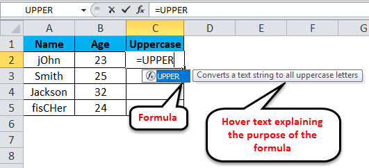
Let us look at the below screenshot.
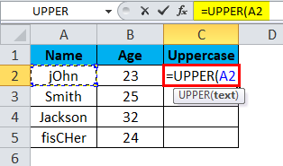
As soon as we enter the text “=upper”, MS Excel automatically displays the formula and the hover text explaining the purpose of the formula. Once we press the ‘Tab’ button, the formula is entered in the cell, and then we need to select the cell whose value we wish to see in the uppercase alphabet. Refer to the screenshot below for more clarity.
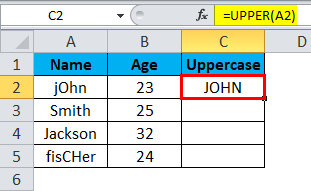
We have selected the cell ‘A2’ (by clicking on it) after we entered the formula in the cell where we wish to get the output. Once the input cell reference (‘A2’ in this case) has been entered, we can close the bracket and press the ‘Enter’ key or simply press the ‘Enter’ key to convert the text into uppercase. The output is shown in the image below.
How to use Uppercase in Excel?
Like every other function/formula we use in MS Excel, we also need to define parameters for ‘Upper’. We cannot enter multiple cell references in the formula of uppercase. However, if more than one word is written in a cell, all the words will get converted to uppercase after executing this formula, as shown in the above image.
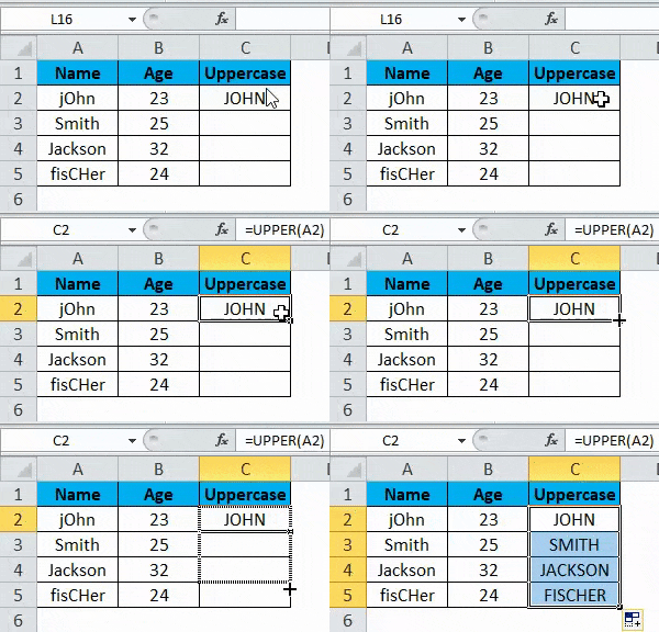
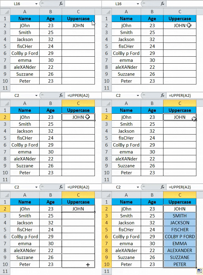
We can use the uppercase formula on multiple cells by dragging it (just like any other formula of MS Excel). Follow the below steps to understand how to use the ‘Upper’ function in MS Excel to convert the alphabet in a cell to the uppercase.
Considering that you have a list of items in column ‘A’ in your Excel file and that cell ‘A1’ is used as the column header, we do not need to capitalize it. This means ‘A2’ will be the first cell we need to capitalize on.
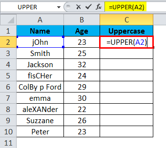
Step 1: Click on the cell where you wish to get the capitalized version of cell ‘A2’. Let us assume it to be ‘C2’ in this case. Enter the formula: “=UPPER(A2)” and hit the enter key.
You will see that the word (or string) written in ‘A2’ is capitalized in ‘C2’.
Step 2: Now, simply click and drag the pointer from C2 to the cell whose values you want to be capitalized. For example, if the list in column A is till ‘A10’, then hold and drag the ‘C2’ column till ‘C10’. (Hold after clicking on the bottom right part of the 1st cell (‘C2 in this case)).
The final output will look like the one shown in the image below.
Things to Remember
The uppercase function in Excel helps you convert the text to all uppercase capital letters.
While applying uppercase in Excel, we need to remember a few things. Some of them are listed below.
1. The’ Upper’ formula accepts only one input parameter.
This formula capitalizes only one cell at a time. We cannot capitalize the entire list in one go with this formula. However, any number of words or strings in the input column will be capitalized in the output with this formula.
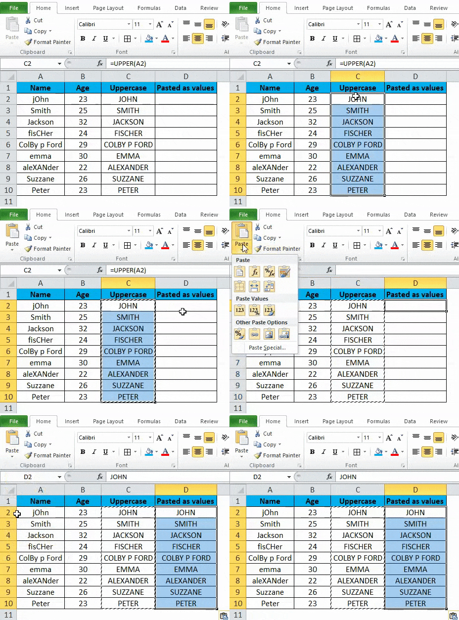
2. After applying the ‘Upper’ formula, if we remove the input list (words), the output list (words) will also be removed.
An easy and direct way to eliminate this problem is by copying the entire contents (i.e., the list) and pasting them as values in the same or any other column. This would ensure that the capitalized values are not deleted. Also, values would appear instead of the formula after we copy and paste values in the column.
Recommended Articles
This has been a guide to Uppercase in Excel. Here we discuss how to convert the words from lowercase to uppercase, along with Excel examples and a downloadable Excel template. You can also go through our other suggested articles –
