Updated August 19, 2023
Excel XOR Function (Table of Contents)
XOR Function in Excel
XOR Functions in Excel perform “Exclusive OR”. This function with two logical statements returns one value. If both statements are TRUE, the result will be FALSE; if any statement is TRUE, then the result will be TRUE.
How to use XOR Function in Excel?
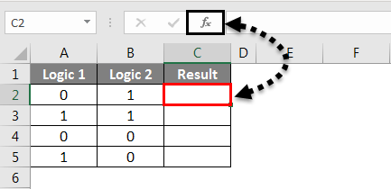
XOR function in Excel can be accessed from the option beside the formula bar with an icon.
Let’s understand how to use XOR Function in Excel by using some examples.
XOR Function in Excel – Example #1
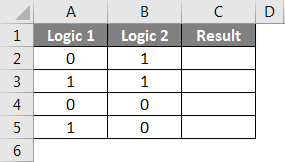
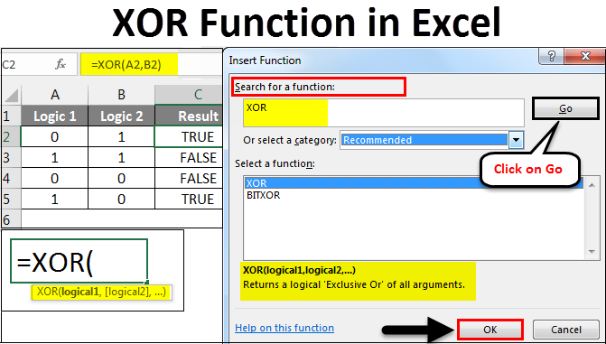
Here we have a table below, wherein columns A and B have some logical values as 0 and 1; on that basis, we need an exclusive answer or result. The result will be the combined results of both logical values. And the result will always be a combination of TRUE or FALSE.
Now to apply XOR Function in Excel, go to the cell where we need to see the result. Now go to the Home menu, and besides the formula bar, click on the Function option with an icon as shown below.
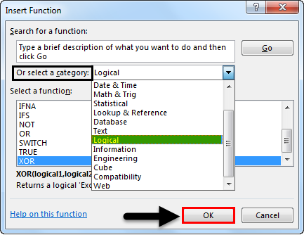
Once we do that, we will get an Insert Function box. Now in Or Select a category option, look for Logical functions, or select All from the drop-down list. And click on OK.
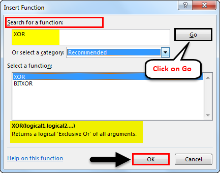
Or else, if the category of the required function is unknown, then Search for a function box. We can search the function XOR with its keyword and click on Go. We will get a possible function below the category list drop-down, as shown below. Then click on OK.
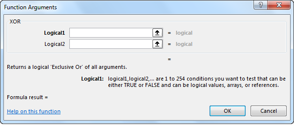
As we can see above, at the bottom of the box, which is highlighted, it has the complete syntax of the selected function from the above list. If the function is completely new, then we can perform the function with the help of syntax in the Insert Function box.
Once we click OK, we will see an argument box of a selected function; as we can see, as per syntax, it asks for logical values as input. We can select any number of logical values.
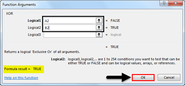
Here, we have selected cells A2 and B2 as our input cells. Once we do that, we will get the suggested result in the argument box at the bottom, as shown below. This shows the correctness of our syntax. After that, click on OK.
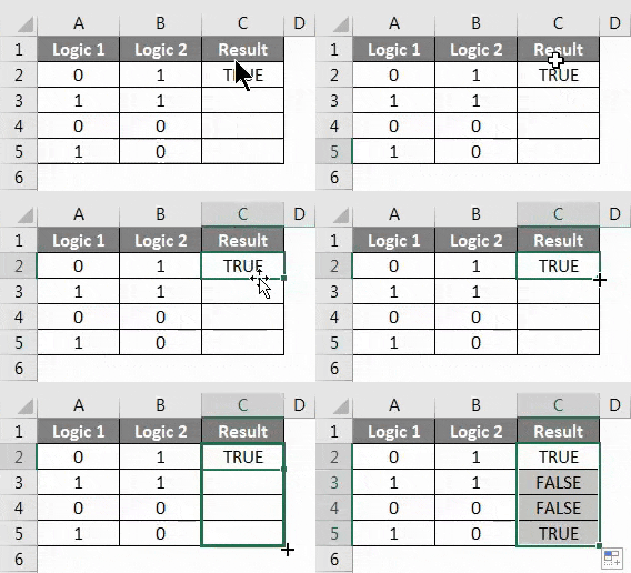
Now drag the formula or apply it to all the selected cells. As shown below, we got an Exclusive-OR value with the help of two logical values.
The logic is simple.
- For two POSITIVE logics, we will get FALSE.
- For two NEGATIVE logics, we will get FALSE.
- If either of them is POSITIVE, we will get TRUE.
This can be applied to any situation where logic is POSITIVE and NEGATIVE.
XOR Function in Excel – Example #2
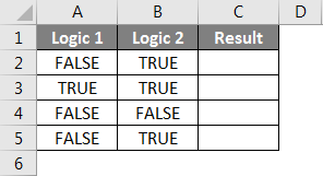
There is one more method of executing the XOR function in Excel, which is easy. Let’s consider a new data set, as shown below. This is a combination of TRUE and FALSE Logics.
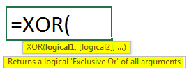
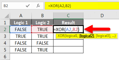
To execute XOR Function in Excel, go to the cell where we want to see the result and type = (Equal) to edit that cell’s edit mode. Once we do that, type or search XOR and select the function as shown below. And we will see the suggested syntax of the selected function, which is boxed in the screenshot below.
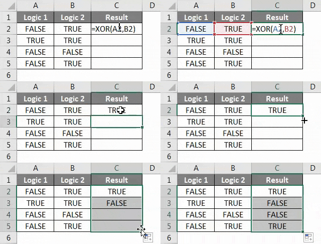
Now select the logical input cells. It can be in any number. We will select cells A2 and B2, as shown below, and press enter to execute the formula. If the syntax is incorrect, then we will get an error.
Once done, drag the formula or syntax in all the related cells, as shown below.
As we can see in the above image, for logic 1 and 2, we got the result in column C. The logic is completely simple, as it was already explained in Example 1.
XOR Function in Excel – Example #3
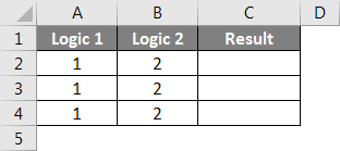
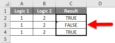
Let’s see an example where we will have 2 logics combined with “1” and “2”, as shown below.
Now for executing XOR for this example, select the cell where we want to see the output and type = (Equal) sign to enable all the functions of Excel and select XOR from the list down as shown below.
Here, we will use the condition of greater than and less than among 1 and 2. Use the combination where 1>0 or 1<0 and the same with 2>0 or 2<0, as shown below.
In the above screenshot, we have used 3 conditions where we showed what the results would be if 1 and 2 are greater and less than 0, respectively, in a different combination. S and below is the actual result.
As we can see above;
- For the 1st condition, where either of one is true, we got TRUE.
- For the 2nd condition, where both are true logic, we got FALSE.
- For the 3rd condition, where either of one is true, we got TRUE, same as Example 1.
Pros
- It is widely used in electronic circuit design for defining the logic before implementation.
- This concept finds versatile application in any context where we encounter scenarios characterized by 0/1, Yes/No, Win/Lose, or True/False outcomes.
- It gives the result based on 2 logic only, and 2 logic can repeat any number of times in any number of cells.
Cons
- The logic-building process sometimes gives the opposite results. So framing correct syntax is necessary.
Things to Remember
- Ensure you are clear with the logic and the required result.
- If text logic is used, use inverted commas quotes (“”) to convert texts into value as text cannot be taken directly in any Excel function.
- Built the logic before using XOR so that when we apply XOR, we can imagine the actual logic with results.
Recommended Articles
This has been a guide to XOR Function in Excel. Here we discussed Using XOR Function in Excel, practical examples, and a downloadable Excel template. You can also go through our other suggested articles –
