Updated August 14, 2023
What is FIND Function in Excel?
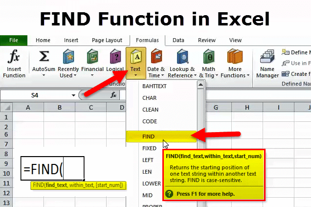
The find function in Excel is an underrated tool that can search for text strings stored in cells and return their positions as output.
The most important thing about the Find function is the cell, which we have taken as a reference, should be in text format. Otherwise, we will get a message as a #Value error message. This also happens; when the Find function cannot find any text in the selected cell, it returns the #Value error again.
FIND Formula in Excel
The FIND formula returns the position of a substring or special character within a text string.
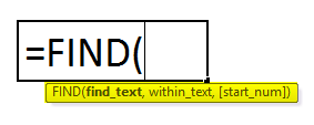
The Formula for the FIND function is as follows:
The first two arguments are mandatory; the last one is optional.
- find_text (required)- the substring or character you want to find.
- within_text (required)- the text string to be searched within. The formula can take the string directly or as a cell reference.
- start_num (optional)- an option that specifies the position in the within_text string or character from which the search should begin.
If excluded, the search starts from the default value 1 of the within_text string.
If the requested find_text is found, the Find function returns a number that represents the position of the within_text. If the supplied find_text is not found, the function returns the Excel #VALUE! Error.
How to Use the FIND Function in Excel?
This FIND Function is very simple and easy to use. Let us now see how to use the Find function with the help of some examples.
Example #1
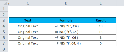
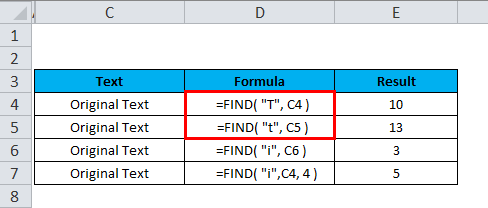
The “Original Text” text string in column C of the spreadsheet uses the Find function to locate different characters.
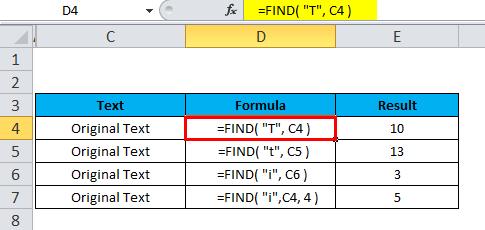
The following formula is used to find the “Original Text” using the FIND function:
Since the Find function is case-sensitive, the lower- and upper-case values, “T” and “t”, give results that are different (for example, in cells D4 & D5).
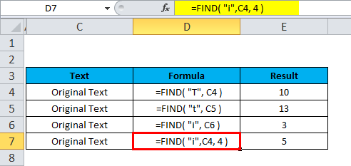
In cell D7, the argument[start_num] is set to 4. Hence the search begins from the fourth character of the within_text string, so the function gives the second instance of the substring “i”.
Example #2
Suppose we wish to find some of the characters from the below data:
- Data is incorrect
- Revenue increased by 5%
- Original Text
Note that in the above spreadsheet:
- Due to the case-sensitive feature of the FIND function, the uppercase find_text value, “T”, will return 3 as its position.
- Since the [start_num] argument is set to 1, the search begins at the first character of the within_text string in cell B8.
Example #3
Find value in a range, worksheet, or workbook.
The below guidelines will let you know how to find text, specific characters, numbers, or dates in a range of cells, worksheets, or the entire workbook.
- To start with, select the range of cells to check-in. To search the whole worksheet, click on any of the cells on the active sheet.
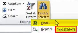
- Open the Find and Replace dialog by pressing the shortcut key Ctrl + F. Alternatively, toggle to the Home tab > Editing group and click Find & Select > Find…
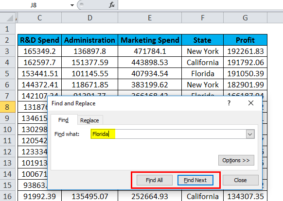
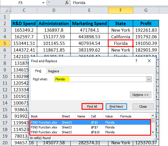
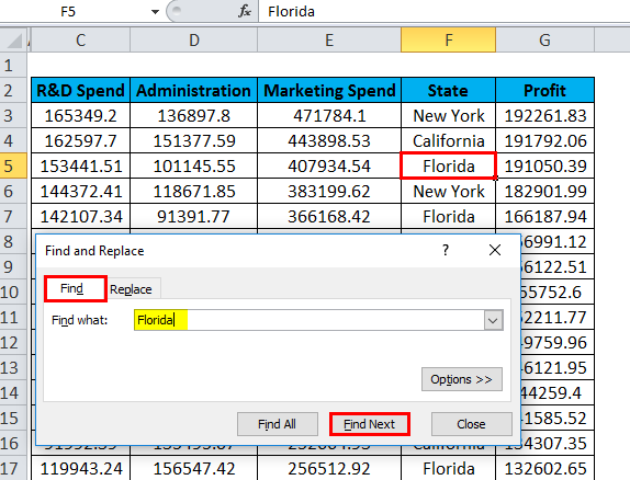
In the Find What box under Find, enter the characters (number or text) you are looking for and click Find All or Find Next.
Clicking on “Find All” will open a list of all occurrences in Excel, and users can navigate to nearby cells by toggling any of the items in the list.
Clicking on Find Next in Excel selects the first occurrence of the search value on the sheet.
FIND Function – additional options:
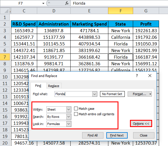
To fine-tune the search, click on the Options in the right-hand corner of Excel’s Find & Replace dialog, and then try any of the below options:
- To search from the active cell from left to right (row-wise), select By Rows in the Search. To check from top to bottom (column-wise), select By Columns.
- To search for a specific value in the entire workbook or current worksheet, select Workbook or Sheet in the Within.
- Select the Match entire cell contents to search for cells with only the characters you entered in the Find what field.
- Search among some data types, Formulas, Values, or Comments in the Look-in.
- For a case-sensitive search, check the Match case check.
Find cells with a specific format in Excel:
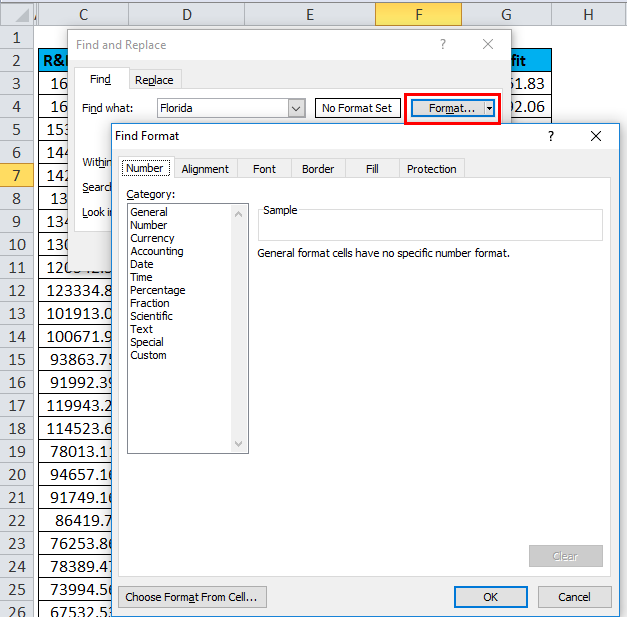
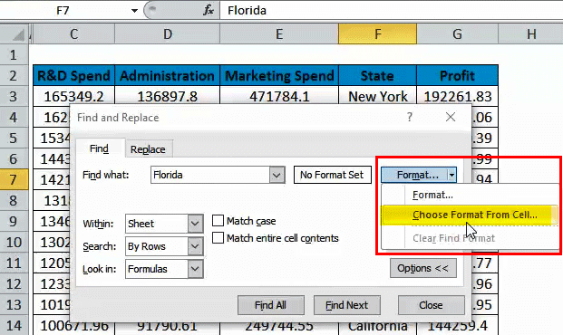
For finding cells with specific formatting, press the shortcut keys Ctrl + F to open the Find and Replace dialog, click Options, then click the Format… button in the upper right corner, and define your selections in the Find Format dialog box.
To find cells that match the format of another cell on your worksheet, delete any criteria in the Find What box, click the arrow next to Format, select Choose Format From Cell, and click the cell with the desired formatting.
FIND Function Error:
If you get an error from the Find function, this will likely be the #VALUE! Error:
Things to Remember
To correctly use the FIND formula, always remember the following simple facts:
- The FIND function is case-sensitive. Use Excel’s SEARCH function if you are looking for a case-insensitive match.
- The FIND function does not permit to use of wildcard characters.
- If the find_text argument contains duplicate characters, the FIND function returns the first character’s position. For example, the formula FIND(“xc”, “Excel”) returns 2 because “x” is the 2nd letter in the word “Excel”.
- If within_text has several occurrences of find_text, the first occurrence is returned. For example, FIND(“p”, “Apple”) returns 2, which is the position of the first “p” character in the word “Apple”.
- If find_text is the string is empty “, the FIND formula returns the first character in the search string.
- The FIND function returns the #VALUE! Error if any of the following occurs:
- Find_text does not exist in within_text.
- Start_num contains more characters than within_text.
- Start_num is 0 (zero) or a negative number.
Recommended Articles
This is a guide to the FIND function in Excel. Here we discuss the FIND Formula and how to use FIND Function in Excel, with practical examples and a downloadable Excel template. You can also go through our other suggested articles –
