Updated May 29, 2023
What are Freeze Columns in Excel?
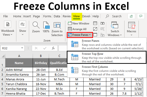
Freeze Columns in Excel can be accessed from the View menu tab’s Window section from the drop-down list of Freeze Panes. Freeze helps us fix the select Column to see the data towards the most right in the worksheet. First, to freeze the column, select the column we want to freeze, put the cursor anywhere in that column, and then select the Freeze Column option from the list. We will be able to see the selected column is now frozen.
Why Freeze Panes?
When you are working on large data, you may be unable to view some of it because it does not fit on the screen. So let’s take a look at the below excel sheet. As you can see in the above screenshot, you can only see columns U and Row 23. So if you have headers in Row 1 and scroll down or right, the headers will not be visible.
This is where Freeze Panes come for help. Freeze panes can keep rows or columns visible while scrolling the rest of the worksheet.
How to Freeze Columns in Excel?
Freeze Panes come with three options, and we will look at them all one by one with examples.
Example #1 – Freeze Top Row
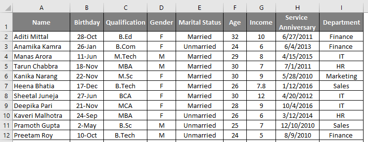
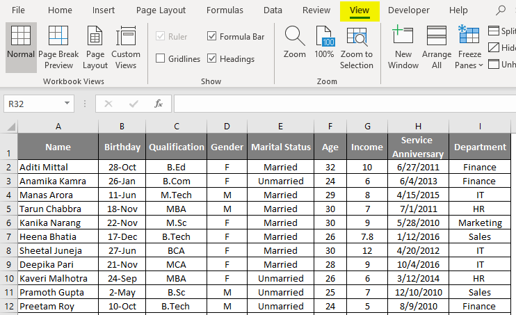
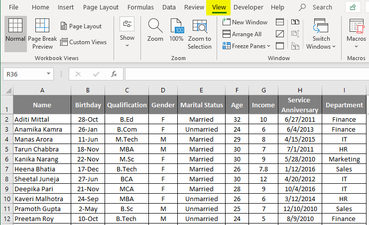
As you can see in the below Excel screenshot, Row 1 is the header for my report, which contains Employee’s personal information, and I want the headers to be visible all the time.
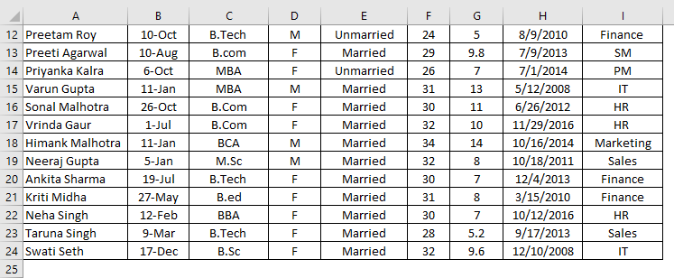
But when I scroll down now, I cannot see the header row.
So to keep the first row visible, I need to Freeze the Top row. To Freeze the top row, we need to execute the following steps:
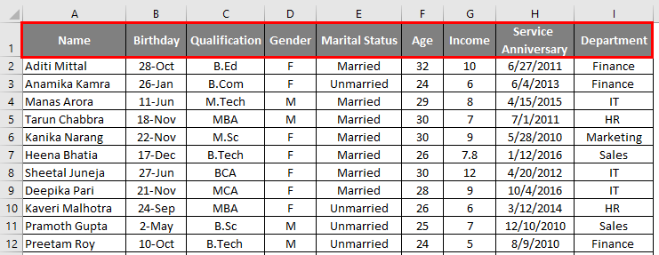
- Select Row 1, as shown in the below screenshot.
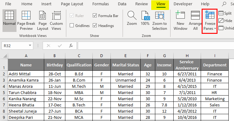
- Go to the View Tab in the Excel Sheet.
- Select Freeze Panes.
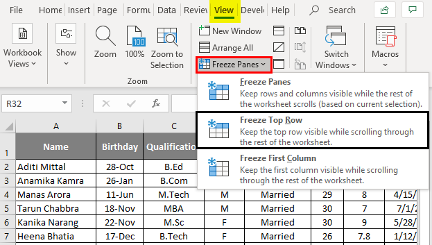
- In the drop-down list, select Freeze Top Row.
- So after selecting Freeze Top Row, you can freeze Row 1 and scroll all the data below Row 1 without losing visibility to the headers.
Example #2 – Freeze the First Column
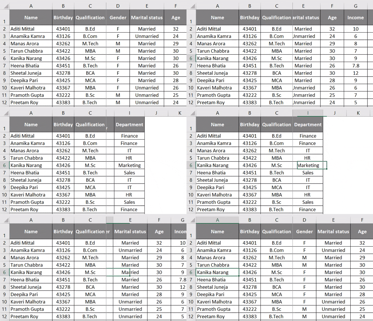
Now, if you have important information in Column A which you want to be visible when you scroll toward the right, you need to use the Freeze the First Column option.
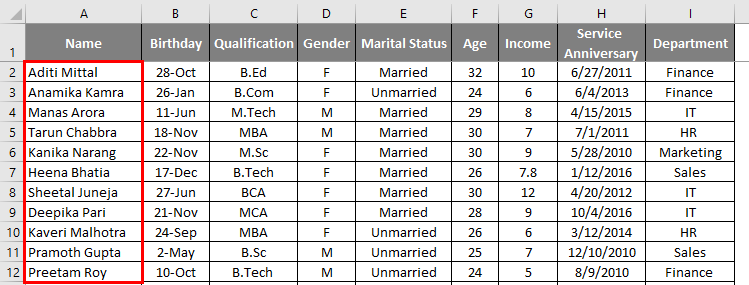
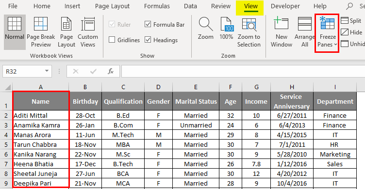
Suppose, in our first example, I want to freeze the Employee Names in Column A. You will need to follow the below steps.
- Select Column A
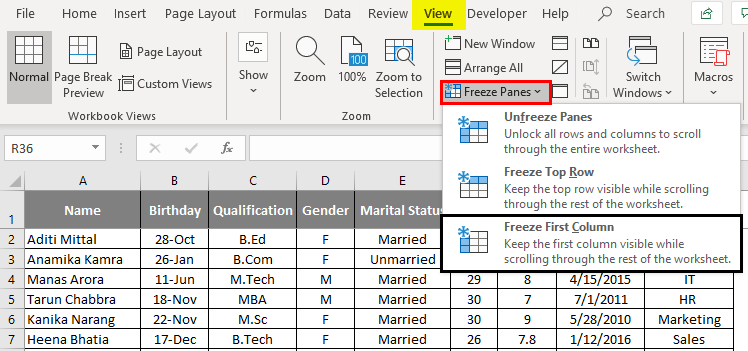
- Go to the View Tab in the Excel Sheet.
- Select Freeze Panes.
In the drop-down list, select Freeze First Column.
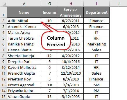
Now when you scroll towards the right, you can scroll without losing visibility to column A.
Example #3 – Freeze Panes
To Freeze any pane in the sheet, whether a row or column, you must select the Freeze Panes option from the drop-down list. This option is not for Top Row and First Column; it will freeze your screen from any row or column you want to freeze and scroll the rest of the data.
You need to follow the below steps to use this option. Go to the View Tab in Excel Sheet and Select Freeze Panes.
- Before selecting the freeze pane, select the cell from where you want to freeze the pane.
- In the below example, if I need to freeze data till Qualification and I want to freeze the top row, I will select cell D2 and click Freeze Panes.
As you can see, data till column C and row 1 is always visible even if you scroll down or scroll toward the right.
How to Unfreeze the Freeze Panes?
If you want to unfreeze the pane and return to the earlier view, follow the steps below.
- Select the Row or Column which is already frozen.
- Go to the View Tab in Excel Sheet and Select Freeze Panes; in the Drop-Down list, select Unfreeze pane so the row or column will be Unfreeze, as shown in the below screenshot.
Things to Remember About Freeze Columns in Excel
- If the Worksheet is in Protected mode, you cannot Freeze or Unfreeze Panes.
- It is very important that while printing anything, you need to Unfreeze the panes as the frozen Rows or Columns will not come while Printing the Worksheet.
- If you are in cell editing mode or page layout view, you cannot Freeze or Unfreeze Panes.
Recommended Articles
This is a guide to Freeze Columns in Excel. Here we discuss how to freeze columns in Excel, practical examples, and a downloadable Excel template. You can also go through our other suggested articles –
