Updated March 27, 2023

Introduction to Gaussian Fit Matlab
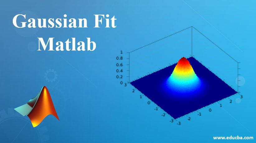
Gaussian fit or Gaussian distribution is defined as a continuous fit that calculates the distribution of binomial events in such a way that the values over the distribution give a probability of 1. The parameters involved in the distribution are mean and the standard deviation. The distribution is in the shape of a bell curve and it was discovered by Carl Friedrich Gauss. There are many applications in real life that follow Gaussian distribution that has a bell fit curve like measuring blood pressure, heights, IQ scores, etc.
Functions of Gaussian Fit in Matlab
In Matlab, we can also use Gaussian fit with different datasets and inputs. The formula is defined as below:
Where a is defined as the amplitude,
- b is the centroid location.
- n is the total number of peaks and it falls in the range of 1 to 8.
- c is given as the width of the peak.
There are various ways of applying the model with Gaussian fit in Matlab like given below:
Gaussian Fit by using “fit” Function in Matlab
The input argument which is used is a Gaussian library model and the functions used are “fit” and “fittype”. The model type can be given as “gauss” with the number of terms that can change from 1 to 8. Please find the below syntax which is used in Matlab for Gaussian fit:
Fi=fit (x, y,” gauss3”)
Gaussian Fit by using Curve Fitting Application:
- Click on cftool and open the Curve Fitting App. We can also click on Curve Fitting from the Apps tab alternatively.
- After that, we need to select the curve fit data i.e. the X data and Y data. By default, the curve fit of the model is Polynomial and we have to change it to Gaussian fit.
- After changing the model type to Gaussian, select the number of terms that needs to be used in the Gaussian fit and it can vary from 1 to 8. We can see the different values of the coefficients, goodness of fit measures and several terms of the model in the Results pane.
- If we want to specify the coefficient starting values, constraint bounds or change the settings of the algorithm, then that can be done in the “Fit Options tab”. Based on the loaded data set, it will also calculate the start points that can be used in the Gaussian models which can be changed manually according to the requirement.
We can also use a Gaussian fit that has an exponential space or has a nonlinear model. They fit the below equation:
Where a, a1, a2 is defined as the amplitude of the peak.
- b, b1, b2 is defined as the centroid of the peak.
- c, c1, c2 is defined as the width of the peak.
The above equation is a nonlinear equation and the coefficients derived are part of an exponential function. Please find the below procedure that is used in applying Gaussian fit to a nonlinear model:
- We have to load the required data set where we want to apply the Gaussian fit. Click on cftool and open the Curve Fitting App. We can also click on Curve Fitting from the Apps tab alternatively.
- The loaded workspace will contain two variables, one of them is a vector of the predictor or independent variable values(xpeak) and the other is a vector of the response or dependent variable values(ypeak). After that, you can select the xpeak for the required X data and ypeak for the required Y data. The fit name that is used here is “Gauss2exp1”.
- After following the above procedure, we have to select Custom Equation for the model and enter the equation with the required terms and input. Currently, the fit is very poor since it contains all the default coefficients with no bounds and starting points are also selected by default.
- Usually, choosing the starting point for the model is easy here since the coefficients used here are straightforward and don’t need any complex interpretation and the exponential background is also well defined. Similarly, mention all the coefficients and constraints for the required model. The parameters which are defined in the above equation like the amplitude of the peak (a, a1, a2) and width of peak (c, c1, c2) cannot be negative in nature. All these parameters can be changed in the Fit Options tab where we have to set the lower bound of the above parameters like the amplitude of the peak and width of peak greater than 0.
Applications of Gaussian Fit
- Gaussian Fit is used in the field of science and engineering to define line emission spectra and chemical concentration.
- It is used in the field of Data Science and Business analytics. Before applying certain models, Gaussian fit or having a bell-shaped curve in important criteria or assumption. It the data is not in the shape of a bell, then we can apply various transformation techniques to the parameters and then apply the model.
- Gaussian fit is also used in the field of Statistics, to define the measures of the normal distribution, Gaussian filters in signal and image processing systems. They are also used to solve the different heat and diffusion equations.
Conclusion
Gaussian fit is an important topic in the field of Statistics and Analytics, where fit is normally in the shape of a bell curve having a standard deviation as an important parameter. There are many properties of Gaussian fit which should be remembered before applying any modeling techniques to the data set.
Recommended Articles
This is a guide to Gaussian Fit Matlab. Here we discuss the introduction and working of Gaussian Fit in Matlab along with applications and function. You may also have a look at the following articles to learn more –


