Introduction to GETPIVOTDATA in Excel
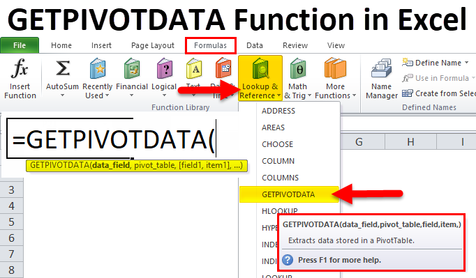
As the name suggests, GETPIVOTDATA means, Get the Data from Pivot Table. It is a kind of pivot table lookup function. It is categorized under the Lookup and Reference function. This function helps in extracting data from specified fields in a Pivot Table. Pivot Table is an analysis tool which summarises a large amount of data in a readable manner.
Getpivotdata can query a pivot table and retrieve specific data based on the table structure instead of the references.
GETPIVOTDATA Formula in Excel
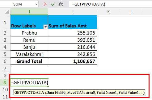
The Formula for the GETPIVOTDATA Function in Excel is as follows:
This function consists of Data Field, Pivot Table, [Field1, Item1], [Field2, Item2], [Field3, Item3].
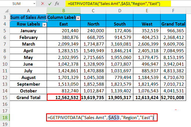
Before explaining, the syntax one by one, let us looks into a simple example.
We are looking for the Grand Total Amount of Region East in the above function.
- Data Field: in the above example, the data field means the heading total you are looking for. In the above example, we are looking for the total sales amount. This is not an optional argument but a required argument.
- Pivot Table: This is a reference to your Data Field cell. In the example shown above, the data filed, i.e. Sales Amt, resides in cell A3, which is why it is taking a reference as A3.
- [Field1, Item1]: We are looking for a Grand Total of Sales Amt for the Region (i.e. [Field1]) East (i.e. Item1).
How to Use GETPIVOTDATA Function in Excel?
GETPIVOTDATA Function in Excel is very simple and easy to use. Let us understand the working of the GETPIVOTDATA Function in Excel with Some Examples.
Example #1
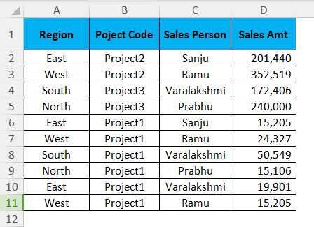
If you have Region in column 1, Project in column 2, Sales Person in column 3, and Sales Values in column 4. You need to get the total of Mr. Sanju using Getpivotdata. Before we apply the function Getpivotdata, firstly, we need to create a pivot table for the below data. Go ahead and apply the function.
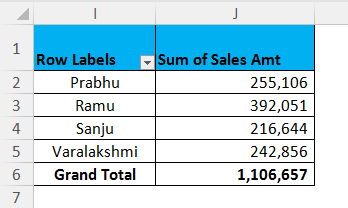
After applying the pivot table, your table should look like this.
Pro Tip: You can apply the Getpivotdata function in Excel in two ways.
- One is by clicking the equal sign (=) in any cell (apart from the pivot table cell) and selecting the desired cell in the pivot table field.
- Secondly, manually enter the formula just like other formulas in Excel.
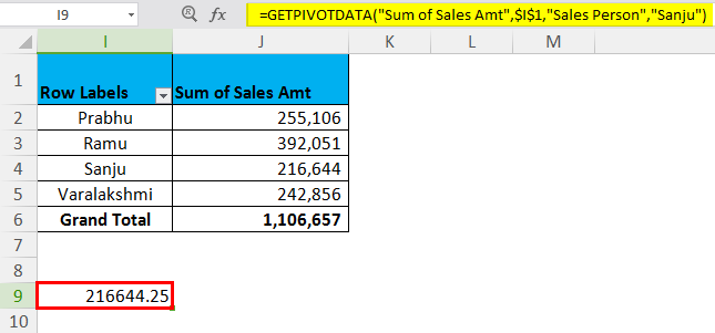
Type 1: Click on any cell and select the desired result cell in the pivot table. This will give you a value of 2,16,444.
Type 2: Enter an equal sign on any cell and enter the Getpivotdata function.
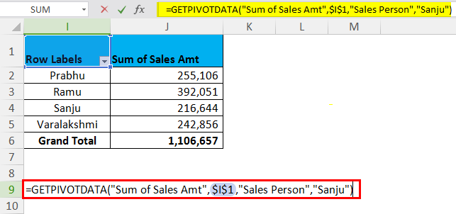
Now in the Data_Field section, type “Sales Amt”. In the Pivot_Table section, type “I1”(reference cell where your Sales Amt resides, in my case, it is I1). In the [Field 1]section, type “Sales Person”, and in [Item1] section, type “Sanju”. This will give you a value of 2,16,444.
Example #2 – Get Pivot Table Sub Totals
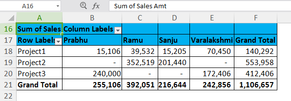
Use the same data table but insert the below kind of pivot table to use the multi-criterion Getpivotdata function. Your pivot should look like this.
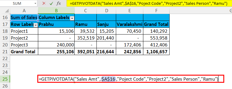
Now the requirement is to get the value of Mr. Ramu for Project 2.
=GETPIVOTDATA(“Sales Amt”,$A$20, “Project Code”, “Project2”, “Sales Person”, “Ramu”)
Data_Field: Sales Amt is the data filed.
Pivot_Table: Cell reference of Sales Amt.
[Filed1] & [Item1]: Project Code is Filed we are looking for, and under project code, we are looking for Project 2.
[Filed2] & [Item2]: Sales Person is filed; we are looking for Ramu under this.
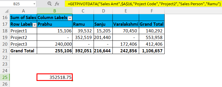
That means we are looking for the total sales amount of Mr. Ramu for Project 2.
Please note the amount of the overall sales for Mr. Ramu is 3,92,051, but for Project 2, it is 3,52,519.
Example #3
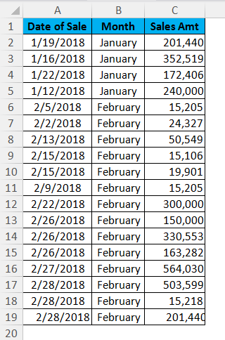
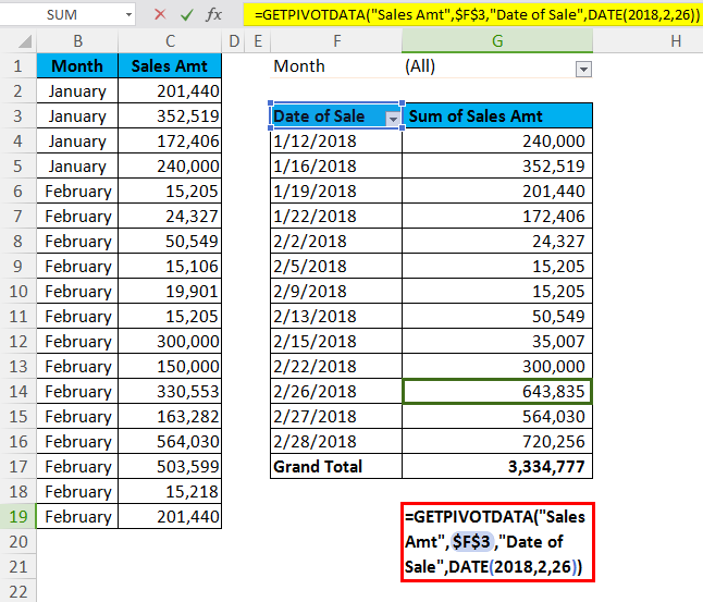
Below is the monthly sales data for Company XYZ. With the use of a pivot table, find the Total Sales Amount for the date 26-02-2018.
Pivot Table Fields & Values
- Apply pivot table for the above data.
- Row data should be Date.
- Value Field should be Sales Amt.
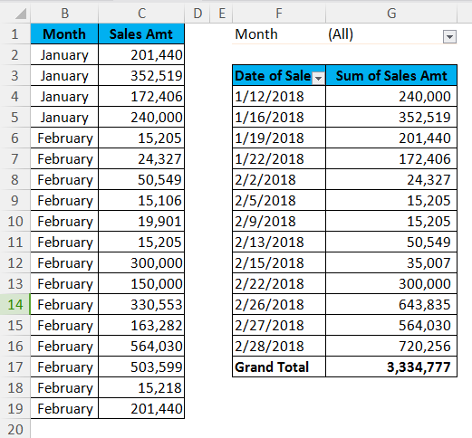
Pivot Table will look like this.
By using this table, find out the sale of 26th Feb 2018.
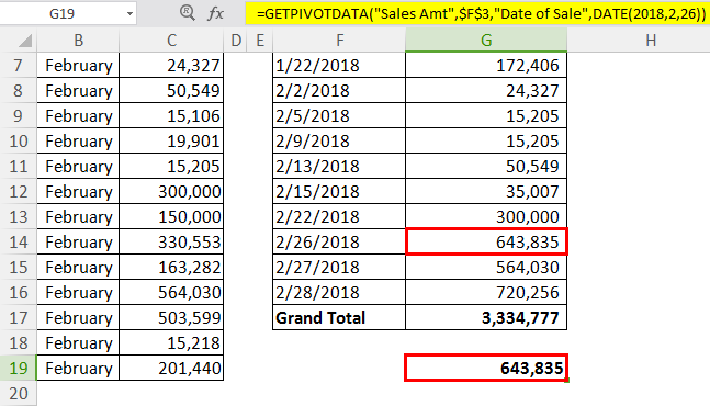
To get a correct answer while typing a date, below is the Getpivotdata Formula.
The sale of 26th Feb 2018 is 643835.
Things to Remember
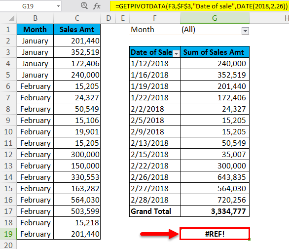
- You cannot change the first argument of the function, i.e. Data_Field, to a cell reference; if so result will throw an error as #REF.
- By default, Excel will take the date format as DATE (2018,2,26), but you change this by just entering the date in “dd-mm-yyyy” format, i.e. “26-02-2018”.
- A function will return a value of #REFerror in case of an incorrect supply of data_field. You cannot give a cell reference to this section.
- All the syntax characters must begin with double quotes (“) and end with the same.
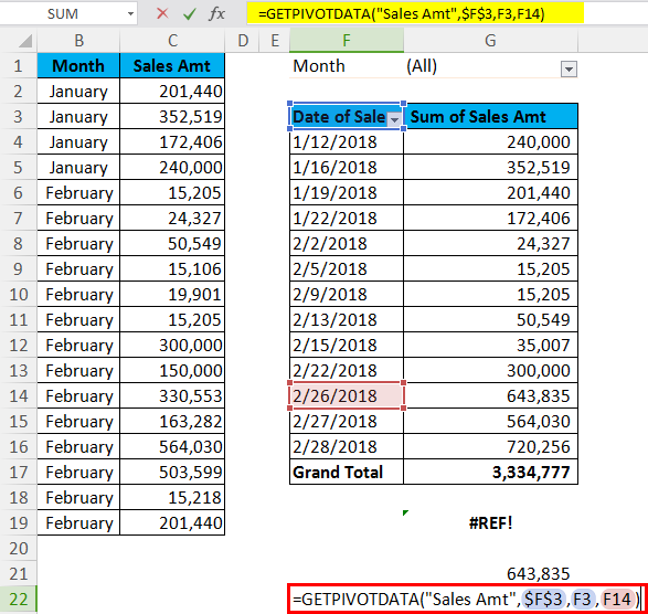
- Apart from data_field for all the remaining fields, we can give a cell reference. This also will give the same result.
- Calculated fields or items and custom calculations are part of this function.
- All the fields should be visible to get the desired result. The function will return a #REF error type if the data is not visible.
- This function will work across the Grand Total & All the Sub Total of the Pivot Table.
Recommended Articles
This has been a guide to GETPIVOTDATA in Excel. Here we discuss the GETPIVOTDATA Formula in Excel and how to use GETPIVOTDATA Function in Excel, along with Excel examples and downloadable Excel templates. You may also look at these useful functions in Excel –
